10.1. Calibration items

Download this page as a Jupyter notebook

This tutorial will focus on performing force calibration using pylake. It is deliberately light on theory, to focus on the practical usage of the calibration procedures. For more theoretical background please refer to the theory section on force calibration.

We can download the data needed for this tutorial directly from Zenodo using Pylake:

filenames = lk.download_from_doi("10.5281/zenodo.7729823", "test_data")

When force calibration is requested in Bluelake, it uses Pylake to perform the calibration, after which a force calibration item is added to the timeline. To see what such items look like, let’s load the dataset:

f = lk.File("test_data/passive_calibration.h5")

The force timeline in this file contains a single calibration measurement. Note that every force axis (e.g. 1x, 1y, 2x, etc.) has its own calibration. We can see calibrations relevant for a single force channel (in this case 1x) by inspecting the calibration attribute for the entire force Slice:

f.force1x.calibration

This returns a list of ForceCalibrationItem instances. In Jupyter notebooks, the following table will also display:

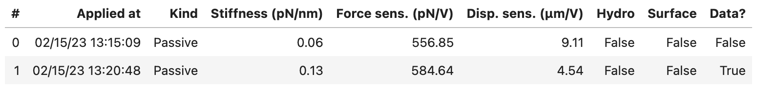
This list provides a quick overview of which calibration items are present in the file and when they were applied. More importantly however, it tells us whether the raw data for the calibration is present in the Slice. When Bluelake creates a calibration item, it only contains the results of a calibration as well as information on when the data was acquired, but not the raw data. We can see this if we plot the time ranges over which these calibration items were acquired and then applied:

plt.figure(figsize=(8, 2))
f.force1x.plot(color='k')
f.force1x.highlight_time_range(f.force1x.calibration[0], color="C0", annotation="0")
f.force1x.highlight_time_range(f.force1x.calibration[0].applied_at, color="C0")
f.force1x.highlight_time_range(f.force1x.calibration[1], color="C1", annotation="1")
f.force1x.highlight_time_range(f.force1x.calibration[1].applied_at, color="C1")

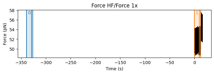
This shows how the calibration items relate to the data present in the file. Calibration item 0 is the calibration that was acquired before the start of this file (and is therefore the calibration that is active when the file starts). Calibration item 1 is the calibration item acquired during the marker saved to this file.

In a Jupyter notebook we can print the details of a specific item:

f.force1x.calibration[1]

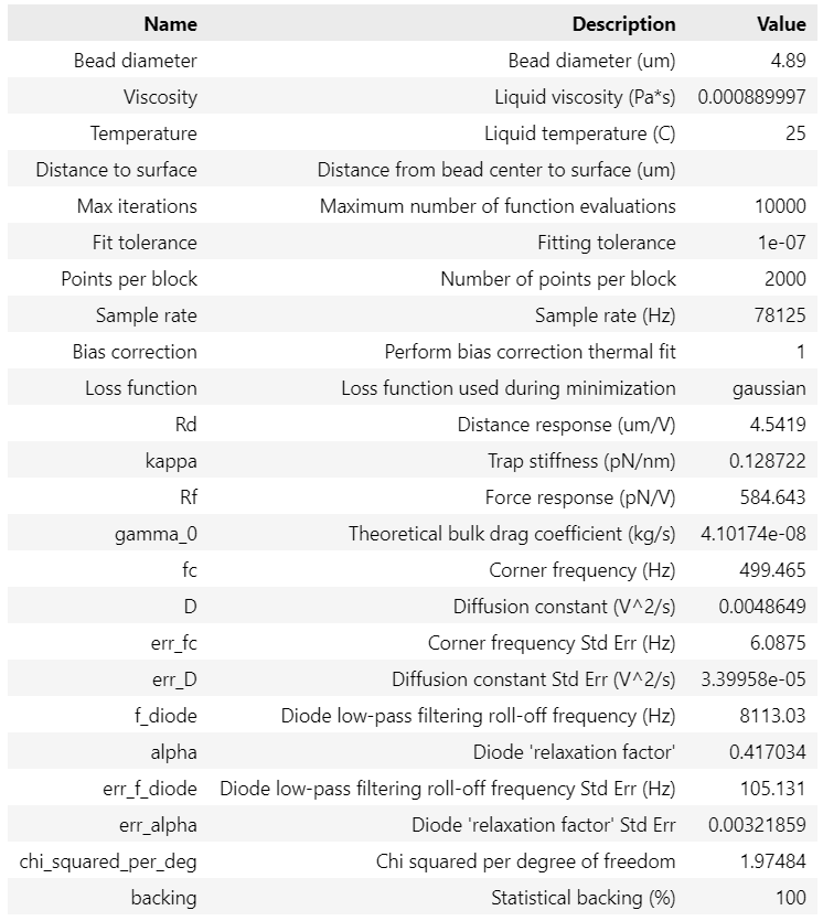
This shows us all the relevant calibration parameters. These parameters are properties and can be extracted as such:

>>> calibration_item = f.force1x.calibration[1]
... calibration_item.stiffness
0.1287225353482303

10.2. Redoing a Bluelake calibration

Starting from Bluelake 2.7.0, it is possible to export the raw data used for calibration with the calibration item. You can enable this in the settings panel in Bluelake. With this feature, recalibrating your data differently becomes a lot easier. If you don’t have this setting enabled, you can still recalibrate your data, but you will have to ensure that you manually export the raw calibration data and slice the appropriate calibration data. To find out how to do this, please refer to the section Recalibrating using timeline data.

10.2.1. Recalibrating using calibration items with raw data

Let’s start by loading our calibration item:

f = lk.File("test_data/raw_data_in_item.h5")
calibration = f.force1x.calibration[0]

We can quickly plot this calibration:

calibration.plot()

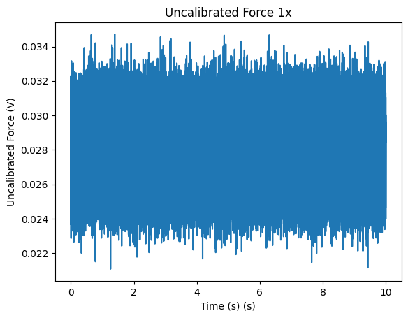
If you wish to obtain the raw calibration data, you can simply access the properties voltage() and for active calibration driving(). These return slices you can plot and interact with:

calibration.voltage.plot()

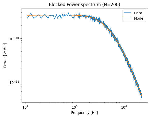
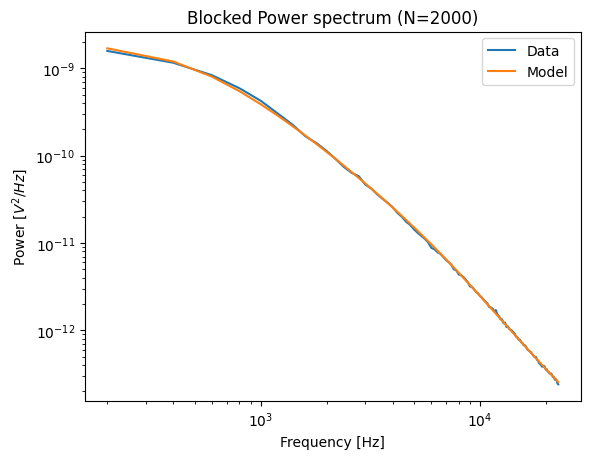
We can easily re-perform this calibration by invoking recalibrate_with(). Let’s see what this spectrum would have looked like with less blocking:

recalibrated = calibration.recalibrate_with(num_points_per_block=200)
recalibrated.plot()

Note that any of the calibration parameters can easily be changed this way. To investigate the effect of the hydrodynamically correct model for example, we can try turning it off:

recalibrated_no_hyco = calibration.recalibrate_with(hydrodynamically_correct=False)
recalibrated_no_hyco.plot()

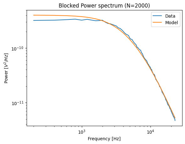
This clearly fits the data poorly. To see what it would do to our timeline data, we can simply recalibrate that by applying the calibration item to recalibrate_force():

recalibrated_force = f.force1x.recalibrate_force(recalibrated_no_hyco)

f.force1x.plot()
recalibrated_force.plot()

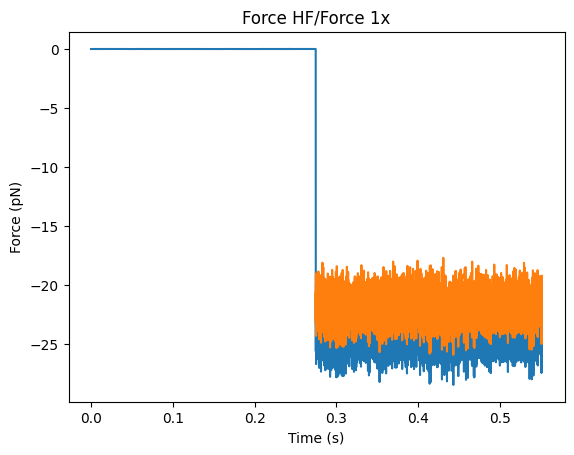
That’s all there is to it.

10.2.2. Recalibrating using timeline data

Important

In order to redo a Bluelake calibration, the force data that was used for the calibration has to be included in the .h5 file. Note that this force data is not exported nor marked by default; it has to be explicitly added to the exported file.

We start by loading the calibration item:

f = lk.File("test_data/passive_calibration.h5")

We can directly slice the channel by the calibration item we want to reproduce to extract the relevant data:

force1x_slice = f.force1x[f.force1x.calibration[1]]

To recalibrate data we first have to de-calibrate the data to get back to raw voltage. To do this, we divide our data by the force sensitivity that was active at the start of the slice.

>>> old_calibration = force1x_slice.calibration[0]
... volts1x_slice = force1x_slice / old_calibration.force_sensitivity

The easiest way to extract all the relevant input parameters for a calibration is to use calibration_params():

>>> calibration_params = f.force1x.calibration[1].calibration_params()
... calibration_params
{'num_points_per_block': 2000,
 'sample_rate': 78125,
 'excluded_ranges': [(19348.0, 19668.0), (24308.0, 24548.0)],
 'fit_range': (100.0, 23000.0),
 'bead_diameter': 4.89,
 'viscosity': 0.00089,
 'temperature': 25.0,
 'fast_sensor': False,
 'axial': False,
 'hydrodynamically_correct': False,
 'active_calibration': False}

This returns a dictionary with the parameters that were set during the calibration in Bluelake. These parameters can be used to reproduce a calibration that was performed in Bluelake by passing these to calibrate_force(). Depending on the type of calibration that was performed, the number of parameters may vary.

Note

If a dictionary of calibration parameters contains parameters named fixed_alpha or fixed_diode this means that your C-Trap has a pre-calibrated diode. In this case, remember that the values for fixed_alpha and fixed_diode depend on the amount of light falling on that trap. If you want to calibrate data corresponding to a different trap power or split, you will need to recalculate these values. For more information, please refer to the diode calibration tutorial.

To quickly reproduce the same calibration that was performed in Bluelake, we can use the function calibrate_force() and unpack the parameters dictionary using the ** notation:

>>> recalibrated = lk.calibrate_force(volts1x_slice.data, **calibration_params)

We can plot this calibration:

recalibrated.plot()

and the residual:

recalibrated.plot_spectrum_residual()

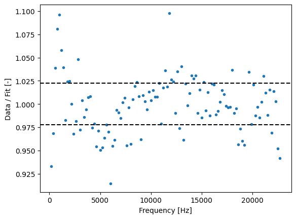
We see that this reproduces the original calibration:

>>> recalibrated.stiffness
0.12872253516809967

>>> f.force1x.calibration[1].stiffness
0.1287225353482303

In this particular case, it looks like we calibrated with the hydrodynamically_correct model disabled:

>>> calibration_params["hydrodynamically_correct"]
False

Given that we used big beads (note the 4.89 micron bead diameter), we should have probably enabled it instead. We can still retroactively change this:

>>> calibration_params["hydrodynamically_correct"] = True
... recalibrated_hyco = lk.calibrate_force(volts1x_slice.data, **calibration_params)
... recalibrated_hyco.stiffness
0.15453110071085924

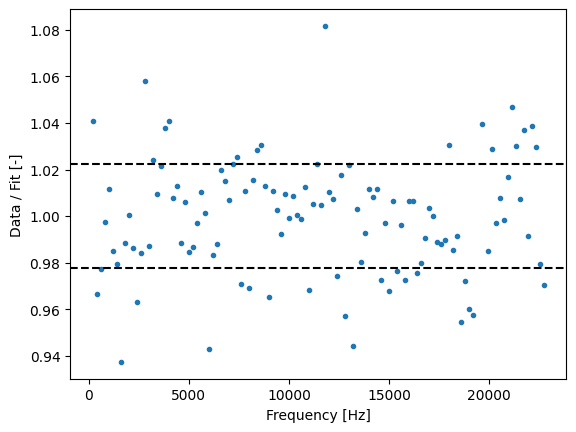
As expected, the difference in this case is substantial. We can also see that the residual now should less systematic deviation:

recalibrated_hyco.plot_spectrum_residual()

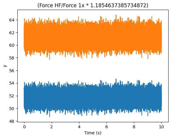
Now that we have our new calibration item, we can recalibrate a slice of force data:

recalibrated_force1x = force1x_slice.recalibrate_force(recalibrated_hyco)

plt.figure()
force1x_slice.plot()
recalibrated_force1x.plot()