Introduction¶

Download this page as a Jupyter notebook

Why is force calibration necessary?¶

Optical tweezers typically measure forces and displacements by detecting deflections of a trapping laser by a trapped bead. These deflections are measured at the back focal plane of the beam using position sensitive detectors (PSDs).

For small displacements $x$ of the bead from the center of the trap, the relation between the force $F$ pulling the bead back towards the center and the displacement can be assumed linear:

\[x = R_d V\]

and

\[F = R_f V\]

Where $V$ is the position-dependent voltage signal from the PSD and $R_d$ and $R_f$ are the displacement and force sensitivity proportionality constants, respectively. Force calibration refers to computing these conversion factors.

Several methods exist to calibrate optical traps based on sensor signals. In this section, we will provide an overview of the physical background of power spectral calibration.

Why does the power spectrum look the way it does?¶

Consider a small bead freely diffusing in a medium (no optical trapping taking place). Neglecting hydrodynamic and inertial effects (more on this later), we obtain the following equation of motion:

\[\dot{x} = \frac{1}{\gamma} F_{thermal}(t)\]

where $x$ is the time-dependent position of the bead, $\dot{x}$ is the first derivative with respect to time, $\gamma$ is the drag coefficient and $F_{thermal}(t)$ is the thermal force driving the diffusion. This thermal force is assumed to have the statistical properties of uncorrelated white noise:

\[F_{thermal}(t) = \sqrt{2 \gamma k_B T} \xi(t)\]

where $k_B$ is the Boltzmann constant, $T$ is the absolute temperature, and $\xi(t)$ is normalized white noise.

We can rewrite this in terms of the diffusion constant by using Einstein’s relation $D = k_B T / \gamma$:

\[\dot{x} = \frac{1}{\gamma} \sqrt{2 \gamma^2 D} \xi(t) = \sqrt{2D} \xi (t) \tag{$\mathrm{m/s}$}\]

with the diffusion constant $D$. Note how this constant depends on the drag coefficient.

The expected power spectrum of such free diffusion is given by the following equation:

\[P_\mathrm{diffusion}(f) = \frac{D}{\pi^2 f^2} \tag{$\mathrm{m^2/Hz}$}\]

We can plot this spectrum for different diffusion constants:

f = np.arange(100, 23000)
for diffusion in 10**np.arange(1, 4):
    plt.loglog(f, diffusion / (np.pi**2 * f**2), label=f"D={diffusion} $\mu m^2/s$")

plt.xlabel("Frequency [Hz]")
plt.ylabel("Amplitude [$\mu m^2$/Hz]");
plt.legend()

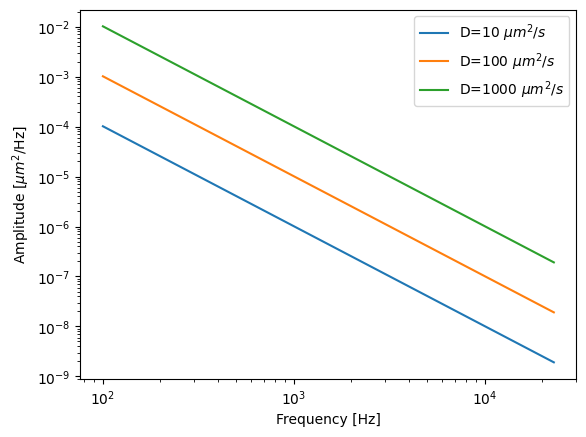
Here, the vertical axis represents a displacement amplitude while the horizontal axis represents frequency. Observe how, for free diffusion, the low frequencies have larger amplitudes than the high frequencies.

Next, consider the effect of the optical trap on this diffusion. The optical trap will pull the bead back towards the focus of the beam. As such, the trap will constrain motion, limiting in particular the high amplitudes. In other words, we expect this effect to be more prominent at low frequencies as they have larger amplitudes. Compared to the previous spectra, this should result in a plateau at the low frequency end of the spectrum. Still neglecting hydrodynamic and inertial effects, one can write down the differential equation for a trapped bead.

\[\dot{x} + \frac{\kappa}{\gamma} x = \sqrt{2D} \xi (t) \tag{$\mathrm{m/s}$}\]

Note that we now have a few additional parameters, namely the drag coefficient $\gamma$ and the trap stiffness $\kappa$. From this, the following power spectrum can be derived:

\[P_{\mathrm{diffusion}}(f) = \frac{D}{\pi^2 \left(f^2 + \left(\frac{\kappa}{2 \pi \gamma}\right)^2\right)} = \frac{D}{\pi^2 \left(f^2 + f_c^2\right) } \tag{$\mathrm{m^2/Hz}$}\]

Note how we’ve defined a corner frequency $f_c$ from the trap stiffness and the drag coefficient. When plotting this equation for various values of the corner frequency, we see the expected plateau:

plt.figure(figsize=(12, 4))
plt.subplot(1, 2, 1)
diffusion, corner_freq = 1000, 1000
for diffusion in 10**np.arange(1, 4):
    plt.loglog(f, diffusion / (np.pi**2 * (f**2 + corner_freq**2)), label=f"D={diffusion} $\mu m^2/s$")

plt.xlabel("Frequency [Hz]")
plt.ylabel("Amplitude [$\mu m^2$/Hz]");
plt.legend()

plt.subplot(1, 2, 2)
diffusion, corner_freq = 1000, 1000
for corner_freq in [1000, 5000, 10000]:
    line, = plt.loglog(
        f, diffusion / (np.pi**2 * (f**2 + corner_freq**2)), label=f"$f_c$={corner_freq} Hz"
    )
    plt.axvline(corner_freq, color=line.get_color(), linestyle="--")

plt.xlabel("Frequency [Hz]")
plt.ylabel("Amplitude [$\mu m^2$/Hz]");
plt.legend()

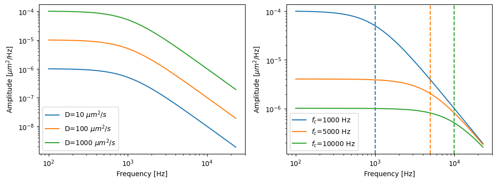
The simple model plotted here is known as the Lorentzian model and it is only a good approximation for small beads (more on that later). We see from the plot that a stiffer trap constrains diffusion more strongly (leading to a wider plateau) and a higher corner frequency. In practice, we wish to fit this spectrum in order to determine the corner frequency which in turn provides information on the trap stiffness once the drag coefficient is known.