Active Calibration¶

Download this page as a Jupyter notebook

For certain applications, passive force calibration, as described above, is not sufficiently accurate. Using active calibration, the accuracy of the calibration can be improved. The reason for this is that active calibration uses fewer assumptions than passive calibration.

When performing passive calibration, we base our calculations on a theoretical drag coefficient. This theoretical drag coefficient depends on parameters that are only known with limited precision:

The diameter of the bead $d$ in microns.
The dynamic viscosity $\eta$ in Pascal seconds.
The distance to the surface $h$ in microns.

This viscosity in turn depends strongly on the local temperature around the bead, which depends on several physical parameters (e.g. the power of the trapping laser, the buffer medium, the bead size and material) and is typically poorly known.

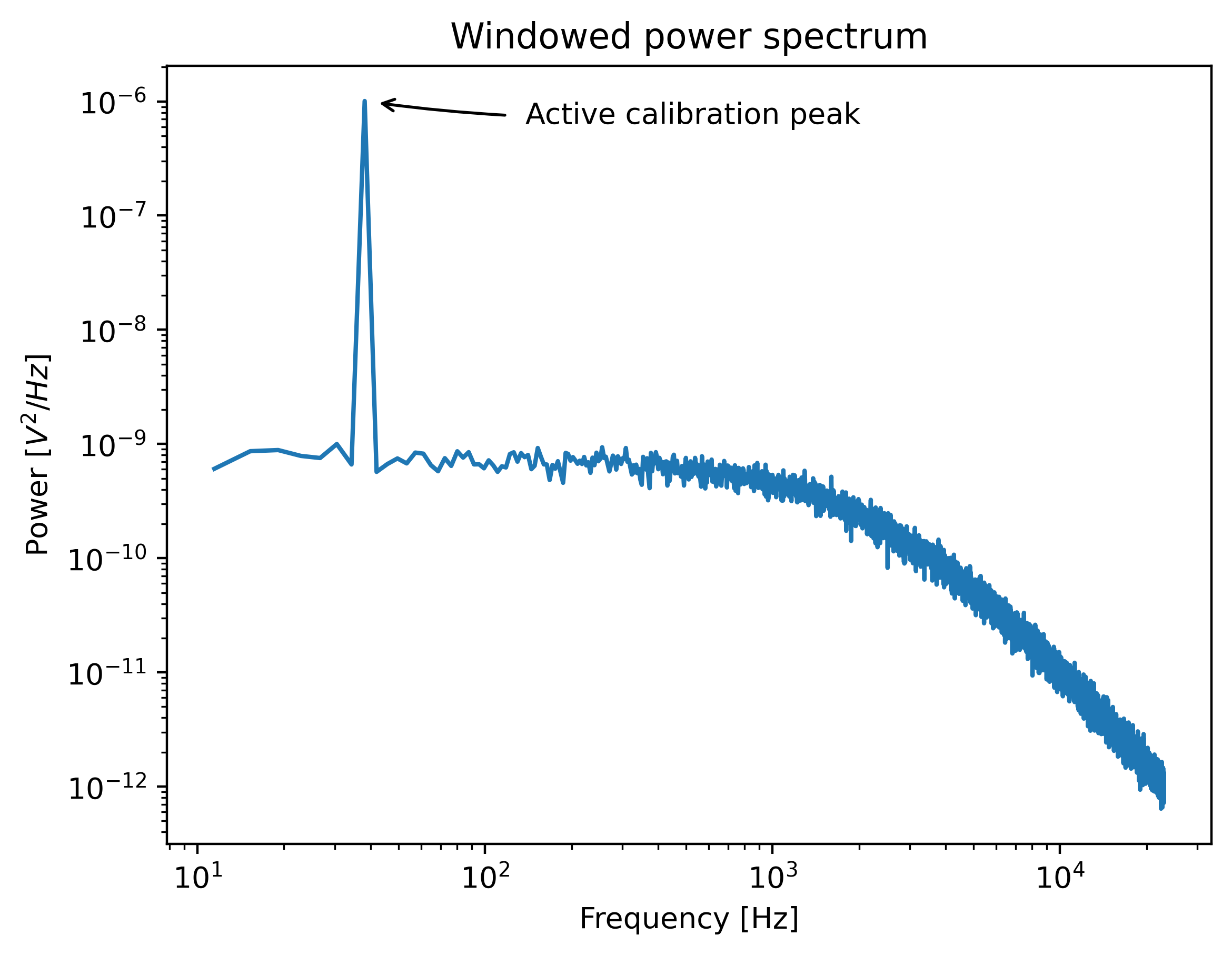
During active calibration, the trap or nanostage is oscillated sinusoidally. These oscillations result in a driving peak in the force spectrum. Using power spectral analysis, the force can then be calibrated without prior knowledge of the drag coefficient.

When the power spectrum is computed from an integer number of oscillations, the driving peak is visible at a single data point at $f_\mathrm{drive}$.

The physical spectrum is then given by a thermal part (like before):

\[P^\mathrm{thermal}(f) = \frac{D}{\pi ^ 2 \left(f^2 + f_c^2\right)} \tag{$\mathrm{m^2/Hz}$}\]

And an active part:

\[P^\mathrm{active}(f) = \frac{A^2}{2\left(1 + \frac{f_c^2}{f_\mathrm{drive}^2}\right)} \delta(f - f_\mathrm{drive}) \tag{$\mathrm{m^2/Hz}$}\]

Here $A$ refers to the driving amplitude. Added together, these give rise to the full power spectrum:

\[P^\mathrm{total}(f) = P^\mathrm{thermal}(f) + P^\mathrm{active}(f) \tag{$\mathrm{m^2/Hz}$}\]

Since we know the driving amplitude, we know how the bead reacts to the driving motion and we can observe this response in the power spectrum, we can use this relation to determine the positional calibration.

If we use the basic Lorentzian model, then the theoretical power (integral over the delta spike) corresponding to the driving input is given by [TolicNorrelykkeSchafferH+06]:

\[W_\mathrm{physical} = \frac{A^2}{2\left(1 + \frac{f_c^2}{f_\mathrm{drive}^2}\right)} \tag{$\mathrm{m^2}$}\]

Subtracting the thermal part of the spectrum, we can determine the same quantity experimentally.

\[W_\mathrm{measured} = \left(P_\mathrm{measured}^\mathrm{total}(f_\mathrm{drive}) - P_\mathrm{measured}^\mathrm{thermal}(f_\mathrm{drive})\right) \Delta f \tag{$\mathrm{V^2}$}\]

where $\Delta f$ refers to the width of one spectral bin. Here the thermal contribution that needs to be subtracted is obtained from fitting the thermal part of the spectrum using the passive calibration procedure from before. The desired positional calibration is then:

\[R_d = \sqrt{\frac{W_\mathrm{physical}}{W_\mathrm{measured}}} \tag{$\mathrm{m/V}$}\]

Note how this time around, we did not rely on assumptions on the viscosity of the medium or the bead size.

As a side effect of this calibration, we actually obtain an experimental estimate of the drag coefficient:

\[\gamma_\mathrm{measured} = \frac{k_B T}{R_d^2 D_\mathrm{measured}} \tag{$\mathrm{kg/s}$}\]

Analogously to passive calibration, there is also a hydrodynamically correct theory for active calibration which should be used when inertial forces cannot be neglected. This involves fitting the thermal spectrum with the hydrodynamically correct power spectrum discussed earlier, but also requires using a hydrodynamically correct model for the peak:

\[P_\mathrm{hydro}^\mathrm{active}(f) = \frac{\left(A f_\mathrm{drive} \left|\gamma / \gamma_0\right|\right)^2 \delta \left(f - f_\mathrm{drive}\right)}{2 \left(\left(f_{c,0} + f \mathrm{Im}(\gamma/\gamma_0) - f^2/f_{m, 0}\right)^2 + \left(f \mathrm{Re}(\gamma / \gamma_0)\right)^2\right)} \tag{$\mathrm{m^2/Hz}$}\]

We can also include a distance to the surface like before. This results in an expression for the drag coefficient $\gamma$ that depends on the distance to the surface which is given by the same equations as listed in the section on the hydrodynamically correct model.

Bead-bead coupling¶

Warning

The implementation of the coupling correction models is still alpha functionality. While usable, this has not yet been tested in a large number of different scenarios.

The active calibration method presented in the previous sections relies on oscillating the nanostage with a known amplitude and frequency. The fluid in the flow-cell follows the stage motion. This in turn exerts a drag on the bead that leads to a sinusoidal displacement of the bead from the trap center. The amplitude of the detected displacement (measured in Volts) and the stage amplitude are then quantified. From the stage amplitude (measured in microns, since the stage position is calibrated) an expected bead displacement is calculated.

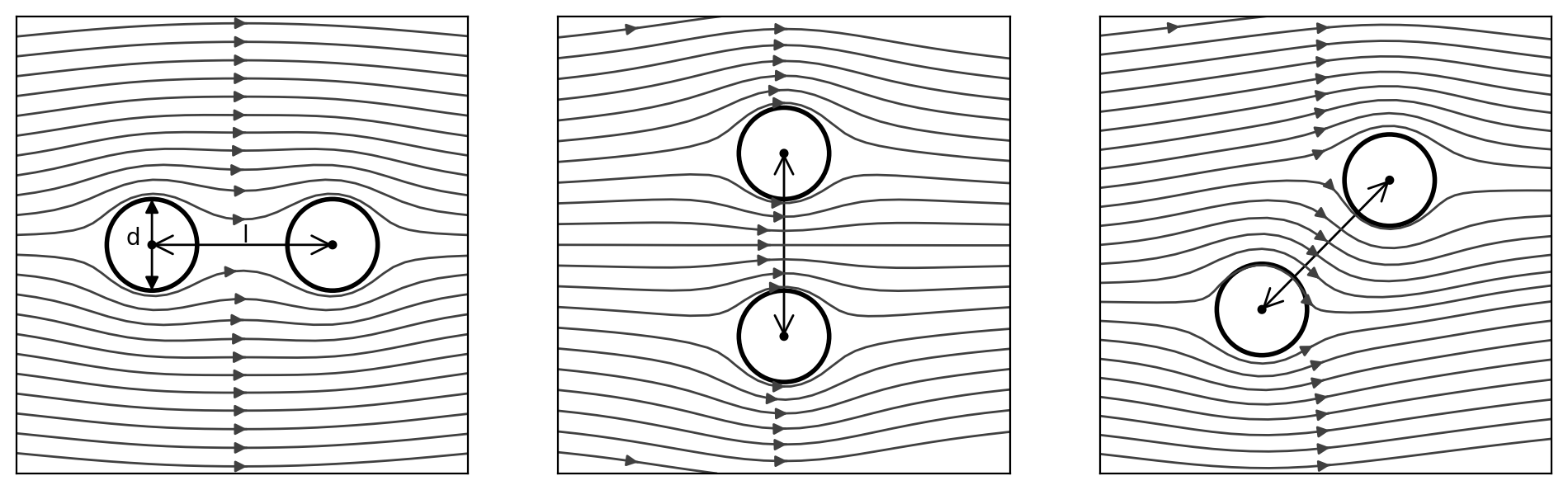
When using two beads, the flow field around the beads is reduced (because the presence of the additional bead slows down the fluid). The magnitude of this effect depends on the bead diameter, distance between the beads and their orientation with respect to the fluid flow. Streamlines for some bead configurations are shown below (simulated using FEniCSx [Dev23]).

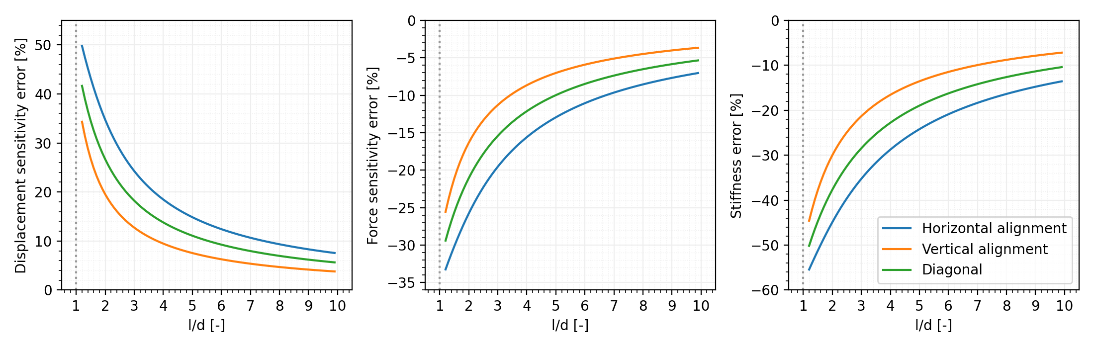
As a result, the bead moves less than expected for a given stage motion.

Since the displacement sensitivity (microns/V) is given by the ratio of the expected bead displacement (in microns) to detected displacement (in Volts) and we detected less displacement than expected (lower voltage amplitude), we obtain an artificially higher displacement sensitivity than expected.

If we define a factor $c$ by which the velocity is reduced, we obtain the following relations for correcting for this reduced flow field:

\[\begin{split}\begin{align} R_{d\mathrm{, corrected}} & = c R_d\\ R_{f\mathrm{, corrected}} & = \frac{1}{c} R_f\\ \kappa_\mathrm{corrected} & = \frac{1}{c^2}\kappa \end{align}\end{split}\]

Where $R_d$ is the displacement sensitivity, $R_f$ is the force sensitivity and $\kappa$ is the stiffness. As shown in the plot below, failing to account for this effect can result in substantial calibration error.

To calculate the desired correction factor $c$, we need to determine what happens to the fluid around the beads. Considering the fluid velocity and viscosity, we can conclude that we typically operate in the regime where viscous effects are dominant (creeping flow). This can be checked by calculating the Reynolds number for the flow. Filling in the maximal velocity we expect during the oscillation, we find the following expression.

\[Re = \frac{\rho u L}{\eta} = 2 \pi f A d \frac{\rho}{\eta}\]

Here $\rho$ refers to the fluid density, $u$ the characteristic velocity, $L$ the characteristic length scale, $\eta$ the viscosity, $f$ the oscillation frequency, $A$ the oscillation amplitude and $d$ the bead diameter. For microfluidic flow, this value is typically much smaller than 1.

In this limit, the Navier-Stokes equation describing fluid flow reduces to the following expressions:

\[\begin{split}\begin{align} \nabla^2 v & = \frac{1}{\eta} \nabla p \\ \nabla \cdot v & = 0 \end{align}\end{split}\]

Here $\eta$ is the viscosity, $p$ is the pressure and $v$ is the fluid velocity. Creeping flow is far removed from every day intuition as it equilibrates instantaneously. The advantage of this is that for sufficiently low frequencies, the correction factor can be based on the correction factor one would obtain for a steady state constant flow.

For two beads aligned in the flow direction, we can use the analytical solution presented in [SJ26]. This model uses symmetry considerations to solve the creeping flow problem for two solid spheres moving at a constant velocity parallel to their line of centers. We denote the correction factor obtained from this model as $c_{\|}$. This correction factor is given by the ratio of the drag coefficient by the drag coefficient one would expect from a single bead in creeping flow ($3 \pi \eta d v$). For beads aligned perpendicular to the flow direction, we use a model from [GCB66], which we denote as $c_{\perp}$.

From the derivations in these papers, it follows that the correction factors obtained depend on the bead diameter(s) $d$ and distance between the beads $l$. For equally sized beads, this dependency is a function of the ratio of the distance between the beads over the bead diameter.

Considering the linearity of the equations that describe creeping flow [GCB66], we can combine the two analytical solutions by decomposing the incoming velocity (in the direction $\vec{e}_{osc}$) into a velocity perpendicular to the bead-to-bead axis $\vec{e}_{\perp}$ and a velocity component aligned with the bead-to-bead axis $\vec{e}_{\|}$.

\[\begin{split}\begin{align} v_{\|} & = (\vec{e}_{\|} \cdot\vec{e}_\mathrm{osc}) c_{\|}\\ v_{\perp} & = (\vec{e}_{\perp} \cdot \vec{e}_\mathrm{osc}) c_{\perp} \end{align}\end{split}\]

This provides us with contributions for each of those axes, but we still need to project this back to the oscillation axis (since this is where we measure our amplitude). We can calculate our desired hydrodynamic correction factor as:

\[c_\mathrm{total} = v_{\|} (\vec{e}_{\|} \cdot \vec{e}_\mathrm{osc}) + v_{\perp} (\vec{e}_{\perp} \cdot \vec{e}_\mathrm{osc})\]

The response of this combined model for equally sized beads can be calculated as follows:

diameter = 1.0
l_d = np.arange(1.01, 8, 0.1) * diameter
zeros = np.zeros(l_d.shape)
plt.plot(l_d, lk.coupling_correction_2d(l_d, zeros, diameter, is_y_oscillation=False), label="horizontal alignment [Stimson et al]")
plt.plot(l_d, lk.coupling_correction_2d(zeros, l_d, diameter, is_y_oscillation=False), label="vertical alignment [Goldman et al]")
plt.plot(l_d, lk.coupling_correction_2d(l_d / np.sqrt(2), l_d / np.sqrt(2), diameter, is_y_oscillation=False), label="diagonal alignment")
plt.ylabel('Correction factor [-]')
plt.xlabel("l/d [-]")
plt.legend()

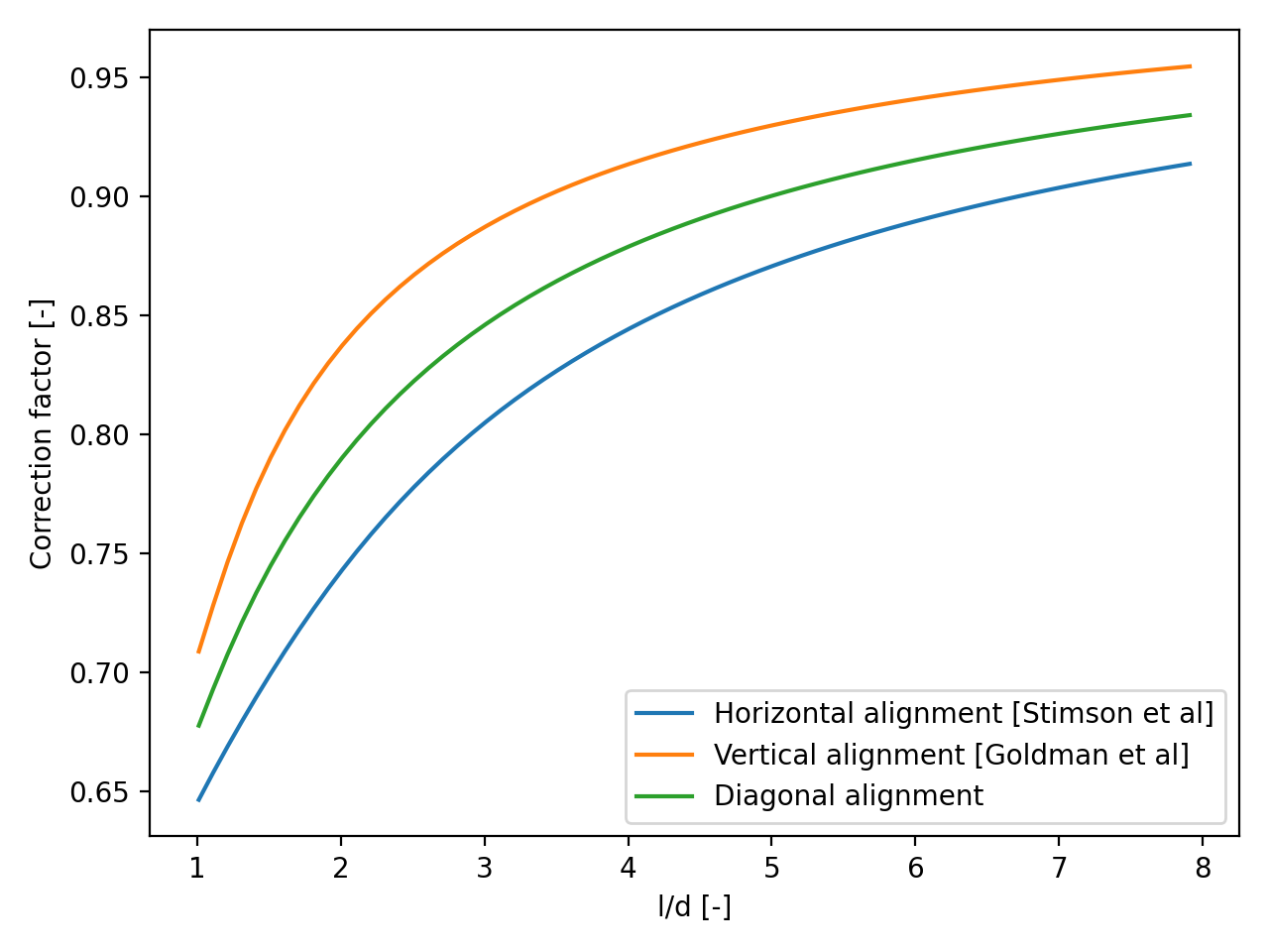
Here, when providing only a horizontal distance recovers the Stimson model [SJ26], while a vertical displacement recovers the Goldman model [GCB66]. To find out more about how to use these correction factors, please refer to the tutorial.