10.5. Active calibration
Download this page as a Jupyter notebook
Pylake can be used to (re-)calibrate the force channels using active calibration data. In active calibration, the stage is oscillated with a known frequency and amplitude. This introduces an extra peak in the power spectrum which allows the trap to be calibrated in a way that relies less on the theoretical drag coefficient. This is particularly useful when the distance to the surface, the bead radius, or the viscosity of the solution is not known accurately. Using Pylake, the procedure to use active calibration is not very different from passive calibration. However, it does require some additional data channels as inputs.
10.5.1. Active calibration with a single bead
Let’s analyze some active calibration data acquired near a surface. We will consider that the nanostage was used as driving input. To do this, load a new file:
lk.download_from_doi("10.5281/zenodo.7729823", "test_data")
f = lk.File("test_data/near_surface_active_calibration.h5")
We decalibrate the force, and extract some relevant parameters:
volts = f.force1x / f.force1x.calibration[0].force_sensitivity
bead_diameter = f.force1x.calibration[0].bead_diameter
# Calibration performed at 1.04 * bead_diameter
distance_to_surface = 1.04 * bead_diameter
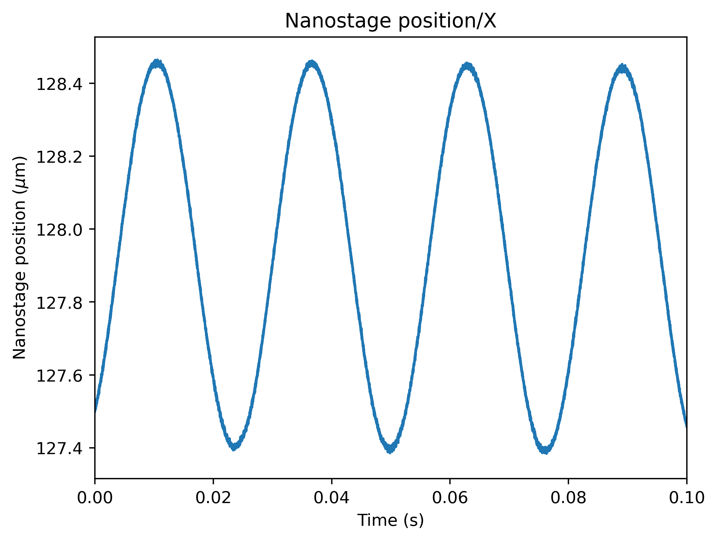
First we need to extract the nanostage data which is used to determine the driving amplitude and frequency:
driving_data = f["Nanostage position"]["X"]
For data acquired with active calibration in Bluelake, this will be a sinusoidal oscillation. If there are unexplained issues with the calibration, it is a good idea to plot the driving signal and verify that the motion looks like a clean sinusoid:
plt.figure()
driving_data.plot()
plt.xlim(0, 0.1)
plt.ylabel(r"Nanostage position ($\mu$m)")
plt.show()
When calibrating actively, we also need to provide the sample rate at which the data was acquired, and a rough guess for the driving frequency. Pylake will find an accurate estimate of the driving frequency based on this initial estimate (provided that it is close enough):
calibration = lk.calibrate_force(
    volts.data,
    bead_diameter=bead_diameter,
    temperature=25,
    sample_rate=volts.sample_rate,
    driving_data=driving_data.data,
    driving_frequency_guess=38,
    distance_to_surface=distance_to_surface,
    num_points_per_block=200,
    active_calibration=True,
    driving_sample_rate=driving_data.sample_rate,
)
We can check the determined driving frequency with:
>>> calibration.driving_frequency
38.15193077664462
Let’s have a look to see if this peak indeed appears in our power spectrum.
To show the peak, we can pass show_active_peak=True to the plotting function of our calibration:
calibration.plot(show_active_peak=True)
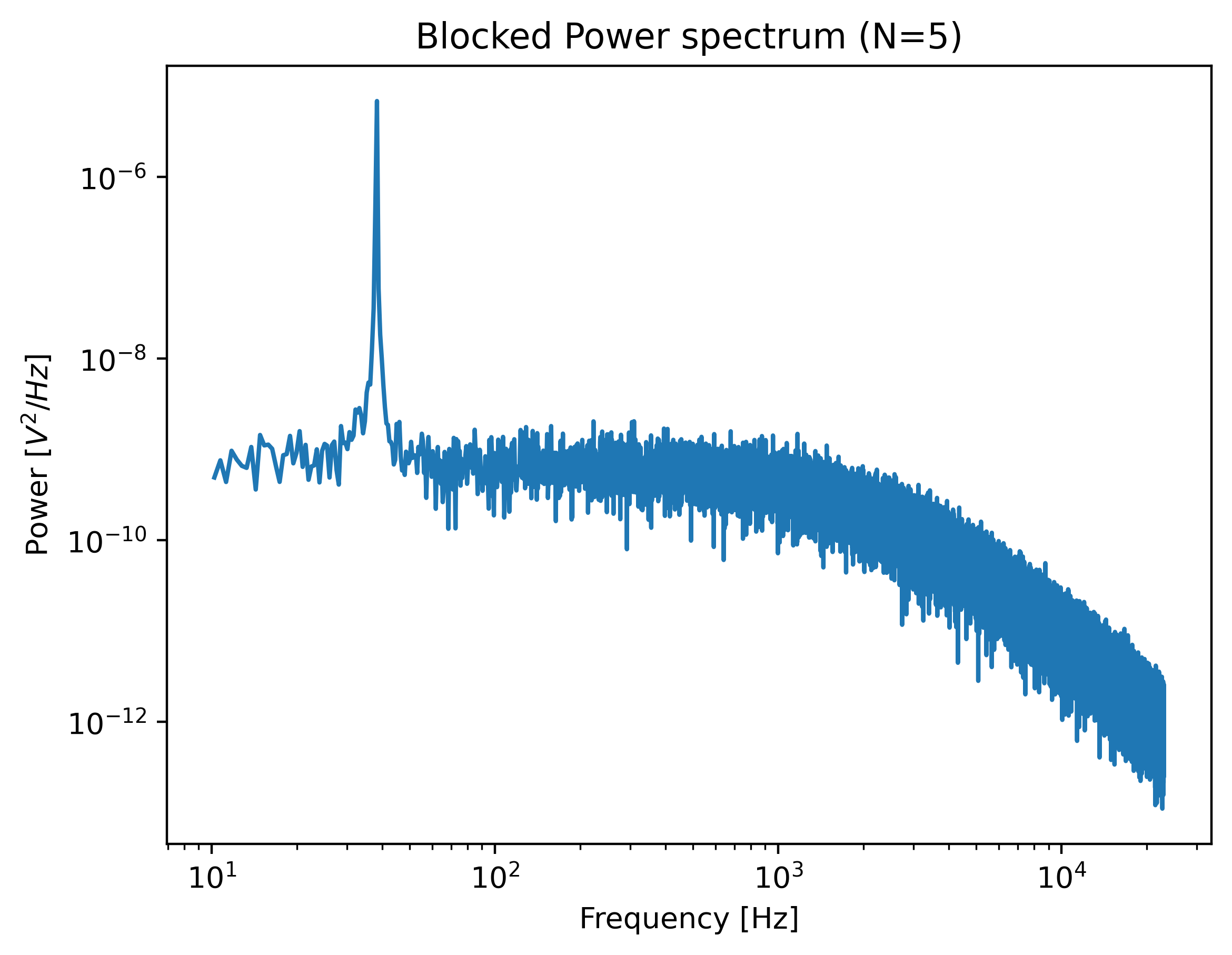
The driving peak is clearly visible in the spectrum. The calibration is now complete and we can access the calibration parameters as before:
>>> print(calibration.stiffness)
0.11637860957657106
Note
Note that the drag coefficient measured_drag_coefficient
that Pylake returns always corresponds to the drag coefficient extrapolated back to its bulk value.
This ensures that drag coefficients can be compared and carried over between experiments performed at different heights.
The field local_drag_coefficient contains an
estimate of the local drag coefficient (at the provided height).
10.5.2. Comparing active calibration to passive
Let’s compare the active calibration result to passive calibration:
>>> passive_fit = lk.calibrate_force(
...     volts.data,
...     bead_diameter=bead_diameter,
...     temperature=25,
...     sample_rate=volts.sample_rate,
...     distance_to_surface=distance_to_surface,
...     num_points_per_block=200
... )
>>> print(passive_fit.stiffness)
0.11751264110743381
This value is quite close to that obtained with active calibration above.
In this experiment, we accurately determined the distance to the surface, but in most cases, this surface is only known very approximately. If we do not provide the height above the surface, we can see that the passive calibration result suffers much more than the active calibration result (as passive calibration fully relies on a drag coefficient calculated from the physical input parameters):
>>> passive_fit = lk.calibrate_force(
...     volts.data,
...     bead_diameter=bead_diameter,
...     temperature=25,
...     sample_rate=volts.sample_rate,
...     num_points_per_block=200
... )
>>> print(passive_fit.stiffness)
0.0860734724588009
10.5.3. Active calibration with two beads far away from the surface
Warning
The implementation of the coupling correction models is still alpha functionality. While usable, this has not yet been tested in a large number of different scenarios. The API can still be subject to change without any prior deprecation notice! If you use this functionality keep a close eye on the changelog for any changes that may affect your analysis.
When performing active calibration with two beads, there is a lower fluid velocity around the beads than there would be with a single bead. This leads to a smaller voltage readout than expected and therefore a higher displacement sensitivity (microns per volt). Failing to take this into account results in a bias. Pylake offers a function to calculate a correction factor to account for the lower velocity around the bead.
Note
For more information on how these factors are derived, please refer to the theory section on this topic.
Appropriate correction factors for oscillation in \(x\) can be calculated as follows:
factor = lk.coupling_correction_2d(dx=5.0, dy=0, bead_diameter=bead_diameter, is_y_oscillation=False)
Here dx and dy represent the horizontal and vertical distance between the beads.
Note that these refer to center to center distances (unlike the distance channel in Bluelake, which represents the bead surface to surface distance).
Note that all three parameters have to be specified in the same spatial unit (meters or micron).
The final parameter is_y_oscillation indicates whether the stage was oscillated in the y-direction.
The obtained correction factor can be used to correct the calibration factors:
Rd_corrected = factor * calibration["Rd"].value
Rf_corrected = calibration["Rf"].value / factor
stiffness_corrected = calibration["kappa"].value / factor**2
To correct a force trace, simply divide it by the correction factor:
corrected_force1x = f.force1x / factor
Note
This coupling model neglects effects from the surface. It is intended for measurements performed at the center of the flowcell.
Note
The model implemented here only supports beads that are aligned in the same plane.
It does not take a mismatch in the z-position of the beads into account.
In reality, the position in the focus depends on the bead radius and may be different for the two beads if they slightly differ in size
(see [AMR18] Fig. 3)
At short bead-to-bead distances, such a mismatch would make the coupling less pronounced than the model predicts.