7. Fd Fitting
Download this page as a Jupyter notebook
Pylake is capable of fitting force extension curves using various polymer models. This tutorial introduces these fitting capabilities.
We can download the data needed for this tutorial directly from Zenodo using Pylake.
Since we don’t want it in our working folder, we’ll put it in a folder called "test_data":
filenames = lk.download_from_doi("10.5281/zenodo.7729929", "test_data")
7.1. Models
Pylake has several models implemented that can be used for fitting force extension data. For a full list of models invoke help(lk.fitting.models)
or see Available models. For example, a model that is frequently used for fitting force extension data of double-stranded DNA (dsDNA) is the so-called
extensible worm-like-chain model by Odijk [Odi95]. We can construct this model using the supplied function lk.ewlc_odijk_distance():
>>> model = lk.ewlc_odijk_distance("DNA")
Note that we passed a name to the model, "DNA", which is used to label the fitting parameters.
Print the model equation and its default parameters:
>>> model

Model equation:

d(f) = DNA.Lc * (1 - (1/2)*sqrt(kT/(f*DNA.Lp)) + f/DNA.St)

Parameter defaults:

Name      Value  Unit      Fitted      Lower bound    Upper bound
------  -------  --------  --------  -------------  -------------
DNA/Lp    40     [nm]      True              0.001            100
DNA/Lc    16     [micron]  True            0.00034            inf
DNA/St  1500     [pN]      True                  1            inf
kT         4.11  [pN*nm]   False              3.77              8
As we can see from the model equation, the model is given as distance as a function of force.
Note also how the model name is prefixed to the model specific parameters, forming a key-value pair like so: "name/parameter": value. For example, the persistence length in this model
is now named DNA/Lp.
kT does not have DNA prefixed since it represents the product of the Boltzmann constant times the temperature, and is therefore not model specific.
We can also obtain the parameters as a list:
>>> print(model.parameter_names)

['DNA/Lp', 'DNA/Lc', 'DNA/St', 'kT']
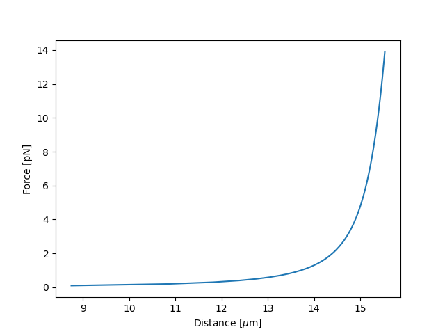
7.2. Simulating the model
We can simulate the model by passing a dictionary with parameters values:
dna = lk.ewlc_odijk_distance("DNA")
force = np.arange(0.1, 14, 0.1)
distance = dna(force, {"DNA/Lp": 50.0, "DNA/Lc": 16.0, "DNA/St": 1500.0, "kT": 4.11})

plt.figure()
plt.plot(distance,force)
plt.ylabel("Force [pN]")
plt.xlabel(r"Distance [$\mu$m]")
plt.show()
7.3. Model composition and inversion
Above, we investigate a model with distance as a function of force. In practice, the force is typically fitted as a function of distance. This can be done using lk.ewlc_odijk_force():
model = lk.ewlc_odijk_force("DNA")
Let’s assume we have acquired data, and upon analysis
we notice that the template matching wasn’t completely optimal. In addition, we experienced some force drift, while
forgetting to reset the force back to zero. In this case, we can incorporate offsets in our model. We can introduce an
offset in the independent parameter, by calling .subtract_independent_offset() on our model:
>>> model = lk.ewlc_odijk_force("DNA").subtract_independent_offset()
>>> model

Model: DNA(x-d)

Model equation:

f(d) = argmin[f](norm(DNA.Lc * (1 - (1/2)*sqrt(kT/(f*DNA.Lp)) + f/DNA.St)-(d - DNA.d_offset)))

Parameter defaults:

Name            Value  Unit      Fitted      Lower bound    Upper bound
------------  -------  --------  --------  -------------  -------------
DNA/d_offset     0.01  [au]      True               -0.1            0.1
DNA/Lp          40     [nm]      True              0.001            100
DNA/Lc          16     [micron]  True            0.00034            inf
DNA/St        1500     [pN]      True                  1            inf
kT               4.11  [pN*nm]   False              3.77              8
If we also expect an offset in the dependent parameter, we can add an offset model to our model:
>>> model = lk.ewlc_odijk_force("DNA").subtract_independent_offset() + lk.force_offset("DNA")
>>> model

Model: DNA(x-d)_with_DNA

Model equation:

f(d) = argmin[f](norm(DNA.Lc * (1 - (1/2)*sqrt(kT/(f*DNA.Lp)) + f/DNA.St)-(d - DNA.d_offset))) + DNA.f_offset

Parameter defaults:

Name            Value  Unit      Fitted      Lower bound    Upper bound
------------  -------  --------  --------  -------------  -------------
DNA/d_offset     0.01  [au]      True               -0.1            0.1
DNA/Lp          40     [nm]      True              0.001            100
DNA/Lc          16     [micron]  True            0.00034            inf
DNA/St        1500     [pN]      True                  1            inf
kT               4.11  [pN*nm]   False              3.77              8
DNA/f_offset     0.01  [pN]      True               -0.1            0.1
Sometimes models become more complicated. For instance, we may have two worm-like chain models, one for a DNA tether and the other for an unfolded protein. The total length of the construct is then the sum of the length of the DNA and the protein and the total distance is given by:
model = lk.ewlc_odijk_distance("DNA") + lk.ewlc_odijk_distance("protein") + lk.distance_offset("offset")
model = model.invert()
Note how the three models all define distance as a function of force. Since fitting is best done for force as a function of distance, we then invert the composited model. Note that models inverted via .invert() will
typically fit slower than the pre-inverted counterparts. This is because the inversion is done numerically rather than
analytically. For example, using lk.ewlc_odijk_force() would be faster to use than lk.ewlc_odijk_distance.invert(). When a pre-inverted function does not exist, as above, using .invert() is the preferred method.
7.4. Fitting data
To fit Fd models, we have to create an FdFit. This object will collect all
the parameters involved in the models and data, and will allow you to interact with the model
parameters and fit them. We construct it using lk.FdFit and pass it one or more models. In
return, we get an object we can interact with, which in this case we store in fit:
model = lk.ewlc_odijk_force("DNA")
fit = lk.FdFit(model)
7.4.1. Adding data to the fit
To do a fit, we have to add data. Let’s assume we have two data sets. One was acquired in the presence of a ligand, and
another was measured without a ligand. We expect this ligand to only affect the contour length of our DNA. Let’s add the
first data set which we name Control. Since the extensible worm-like chain is valid up to 30 pN, we select forces < 30pN:
file1 = lk.File("test_data/fdcurve.h5")
fd1 = file1.fdcurves["FD_5_control_forw"]
mask1 = fd1.f.data <= 30
force1 = fd1.f[mask1].data
distance1 = fd1.d[mask1].data
fit.add_data("Control", force1, distance1)
For the second data set, we want the contour length to be different. We can achieve this by renaming the parameter
when loading the data from DNA/Lc to DNA/Lc_RecA:
file2 = lk.File("test_data/fdcurve_reca.h5")
fd2 = file2.fdcurves["FD_5_3_RecA_forw_after_2_quick_manual_FD"]
mask2 = fd2.f.data <= 30
force2 = fd2.f[mask2].data
distance2 = fd2.d[mask2].data
fit.add_data("RecA", force2, distance2, params={"DNA/Lc": "DNA/Lc_RecA"})
Multiple criteria can be combined into a single mask by using numpy’s logical operators.
For example, to select all forces up to 30 pN and ensure a distance larger than 1.5 micron:
example_mask = np.logical_and(fd1.f.data <= 30, fd1.d.data > 1.5)
Adding a third condition that the distance has to be < 4 micron can be done as follows (note the double brackets):
example_mask = np.logical_and.reduce((fd1.f.data <= 30, fd1.d.data > 1.5, fd1.d.data < 4.0))
7.4.2. Setting parameter bounds
The parameters of the model can be accessed directly from FdFit. Note that by default, parameters tend to have
reasonable initial guesses and bounds in pylake for dsDNA, but we can set our own as follows:
fit["DNA/Lp"].value = 50
fit["DNA/Lp"].lower_bound = 39
fit["DNA/Lp"].upper_bound = 80
fit["DNA/Lc"].value = 2.7
fit["DNA/Lc_RecA"].value = 3
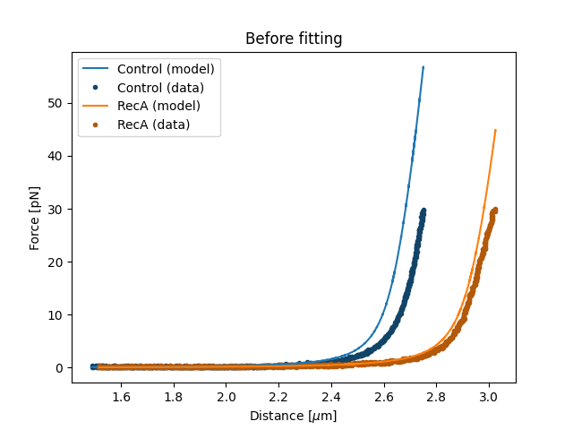
Parameter estimation is typically initiated from an initial guess. A poor initial guess can lead to a poor parameter estimate. Therefore, you might want to see what your initial model curve looks like and set some better initial guesses yourself.:
plt.figure()
fit.plot()
plt.ylabel("Force [pN]")
plt.xlabel(r"Distance [$\mu$m]")
plt.title("Before fitting")
plt.show()
After tuning the initial guesses, the model is ready to be fitted. We can fit the model to the data by calling the
function .fit(). This estimates the model parameters by
minimizing the least squares differences between the model’s dependent variable and the data in the
fit:
fit.fit()
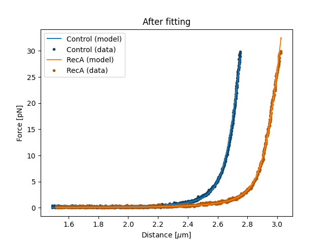
7.5. Plotting the results of the fit
Plot the result of the fit:
plt.figure()
fit.plot()
plt.ylabel("Force [pN]")
plt.xlabel(r"Distance [$\mu$m]");
plt.title("After fitting")
plt.show()
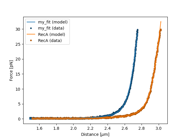
If you wish to customize the label that appears in the legend, you can pass a custom label as an additional argument:
plt.figure()
fit.plot(label="my_fit")
plt.xlabel(r"Distance [$\mu$m]")
plt.ylabel("Force [pN]")
plt.show()
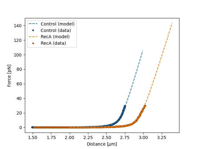
Sometimes, we want to plot the model over a range of
values (in this case values from 2.0 to 5.0) for the conditions corresponding to the Control and RecA data. We can
do this as follows:
plt.figure()
fit.plot("Control", "--", np.arange(2.0, 3.0, 0.01))
fit.plot("RecA", "--", np.arange(2.0, 3.4, 0.01))
plt.xlabel(r"Distance [$\mu$m]")
plt.ylabel("Force [pN]")
plt.show()
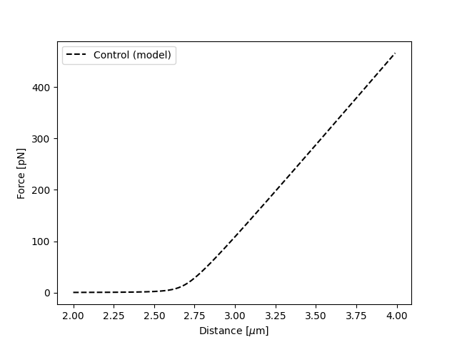
Plot the fitted model without data:
plt.figure()
fit.plot("Control", "k--", np.arange(2.0, 4.0, 0.01), plot_data=False)
plt.xlabel(r"Distance [$\mu$m]")
plt.ylabel("Force [pN]")
plt.show()
It is also possible to obtain simulations from the model directly, using the fitted parameters:
distance = np.arange(2.0, 5.0, 0.01)
simulated_force = model(distance, fit["Control"])
plt.figure()
plt.plot(distance, simulated_force)
plt.xlabel(r"Distance [$\mu$m]")
plt.ylabel("Force [pN]")
plt.show()
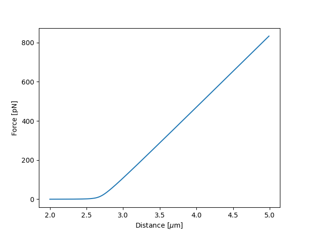
Here fit["Control"] grabs the parameters needed to simulate the condition corresponding to the dataset with the name "Control".
7.6. Incremental fitting
Rather than fitting all conditions at once, fits can also be done incrementally:
>>> model = lk.ewlc_odijk_force("DNA")
>>> fit = lk.FdFit(model)
>>> print(fit.params)
No parameters
We can see that there are no parameters to be fitted. The reason for this is that we did not add any data to the fit yet. Let’s add some and fit this data:
>>> fit.add_data("Control", force1, distance1)
>>> fit.fit()
>>> print(fit.params)
Name         Value  Unit      Fitted      Lower bound    Upper bound
------  ----------  --------  --------  -------------  -------------
DNA/Lp    59.409    [nm]      True              0.001            100
DNA/Lc     2.81072  [micron]  True            0.00034            inf
DNA/St  1322.9      [pN]      True                  1            inf
kT         4.11     [pN*nm]   False              3.77              8
Let’s add a second data set where we expect a different contour length and refit:
>>> fit.add_data("RecA", force2, distance2, params={"DNA/Lc": "DNA/Lc_RecA"})
>>> print(fit.params)
Name              Value  Unit      Fitted      Lower bound    Upper bound
-----------  ----------  --------  --------  -------------  -------------
DNA/Lp         89.3347   [nm]      True              0.001            100
DNA/Lc          2.80061  [micron]  True            0.00034            inf
DNA/St       1597.68     [pN]      True                  1            inf
kT              4.11     [pN*nm]   False              3.77              8
DNA/Lc_RecA     3.7758   [micron]  True            0.00034            inf
We see that indeed the second parameter now appears. We also note that the parameters from the first fit changed. If
this was not intentional, we should have fixed these parameters after the first fit. For example, we can fix the
parameter DNA/Lp by invoking:
>>> fit["DNA/Lp"].fixed = True
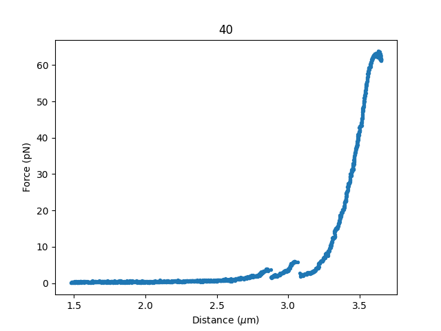
7.7. Calculating per point contour length
Sometimes, one wishes to invert the model with respect to one parameter (i.e. re-estimate one parameter on a per data point basis). This can be used to obtain dynamic contour lengths:
file3 = lk.File("test_data/fd_multiple_Lc.h5")
fd3 = file3.fdcurves["40"]
force3 = fd3.f.data
distance3 = fd3.d.data

plt.figure()
fd3.plot_scatter()
First set up a model and fit it to data without varying contour length:
# Define the model to be fitted
model = lk.ewlc_odijk_force("model") + lk.force_offset("model")

# Fit the overall model first
fit = lk.FdFit(model)
fit.add_data("Control", force1, distance1)
fit.fit()
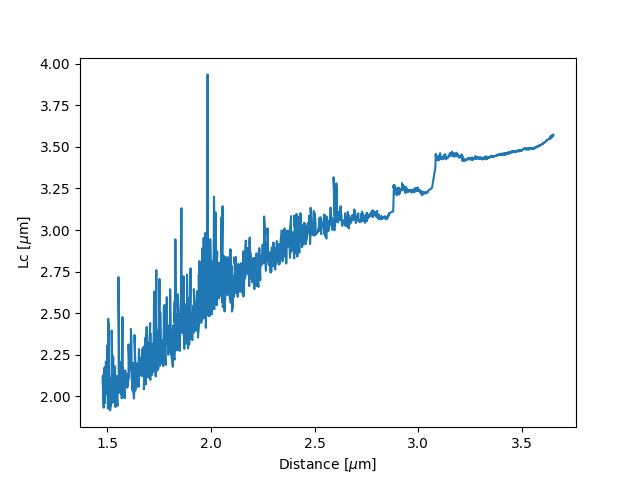
Now, we wish to allow the contour length to vary on a per data point basis. For this, we use the function
parameter_trace():
lcs = lk.parameter_trace(model, fit["Control"], "model/Lc", distance3, force3)
plt.figure()
plt.plot(distance3,lcs)
plt.xlabel(r"Distance [$\mu$m]")
plt.ylabel(r"Lc [$\mu$m]")
plt.show()
Here we see a few things happening. The first argument specifies the model to use for the inversion.
The second argument should contain the parameters to be used in this method. Note how we select them from the parameters
in the fit using the same syntax as before (i.e. fit[data_name]). Next, we specify which parameter has to be fitted
on a per data point basis. Finally, we supply the
data to use in this analysis. First the independent parameter is passed, followed by the dependent parameter.
7.8. Advanced usage
7.8.1. Confidence intervals and standard errors
Once parameters have been fitted, standard errors can be obtained as follows:
>>> fit["model/Lc"].stderr
0.0015047272987879956
Assuming that the parameters are not at the bounds, the sum of random variables with finite moments converges to a
Gaussian distribution. This allows for the computation of confidence intervals using the Wald test
[PT90]. To get these asymptotic intervals, we can use the member function .ci with a desired
confidence interval:
>>> fit["model/Lc"].ci(0.95)
[2.7683400869428114, 2.7742385095671684]
Note that the bounds returned by this call are only asymptotically correct and should be used with caution. Better confidence intervals can be obtained using the profile likelihood method [MHS+16, RKM+09]. Determining confidence intervals via profiles has two big advantages:
The confidence intervals no longer depend on the parametrization of the model (for more information on this see [MHS+16]).
By inspecting the profile, we can diagnose problems with the model we are using.
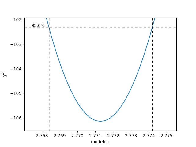
Profiles can easily be computed by calling profile_likelihood() on the fit:
>>> profile = fit.profile_likelihood("model/Lc", num_steps=5000)
[2.768390344105447, 2.774203622954422]
The lower and upper bound of the 95% confidence interval of the given parameter (Lc in this example) can be obtained as:
[profile.lower_bound, profile.upper_bound] # [lower bound, upper bound]
Note that these profiles require iterative computation and are therefore time consuming to produce. For a well parametrized model with sufficient data, a profile plot results in a (near) parabolic shape, where the line of the parabola intersects with the confidence interval lines (dashed). The confidence intervals are then determined to be at those intersection points:
plt.figure()
profile.plot()
plt.show()
Another thing that may be of interest is to plot the relations between parameters in these profile likelihoods:
plt.figure()
profile.plot_relations()
plt.show()
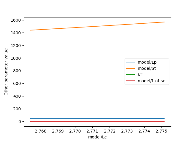
These inferred relations can provide information on the coupling between different parameters. This can be quite informative when diagnosing fitting issues. For example, when fitting a contour length in the presence of an distance offset, we can observe that the two are related. To produce the following figure, we set a lower bound and upper bound of -0.1 and 0.1 for the distance respectively. We can see that the profile is perfectly flat until the distance reaches the bound. Only then does the profile suddenly jump.
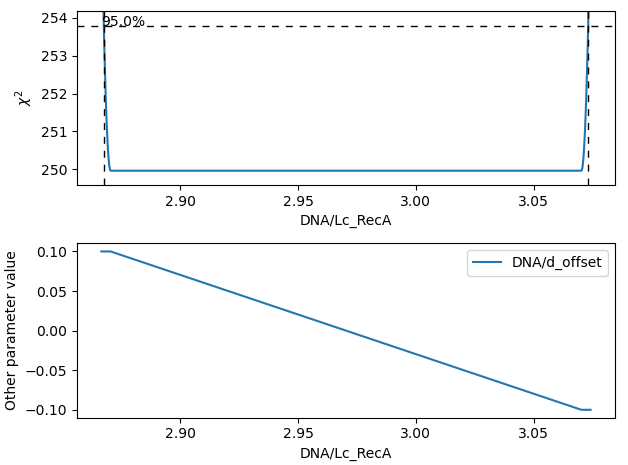
What this shows is that a change in one parameter (model/Lc) can be compensated by a change in the other. This
highlights the importance of constraining distance offset parameters when trying to estimate an absolute contour length.
In this sample case, fixing the distance offset to zero recovers the parabolic profile from before.
7.8.2. Adding many data sets
Sometimes, you may want to add multiple data sets for one condition to perform a global fit.
Consider two lists of distance and force vectors stored in distances and forces:
file_adk1 = lk.File("test_data/adk5_curve1.h5")
d_adk1 = file_adk1.fdcurves["adk5_curve1"].d["0s":"13s"].data
f_adk1 = file_adk1.fdcurves["adk5_curve1"].f["0s":"13s"].data

file_adk2 = lk.File("test_data/adk5_curve2.h5")
d_adk2 = file_adk2.fdcurves["adk5_curve2"]["0s":"13s"].d.data
f_adk2 = file_adk2.fdcurves["adk5_curve2"]["0s":"13s"].f.data

distances = [d_adk1[d_adk1 > 0], d_adk2[d_adk2 > 0]]
forces = [f_adk1[d_adk1 > 0], f_adk2[d_adk2 > 0]]
Note that when beads are not tracked properly, a zero distance is returned. Therefore we only selected data for which the distance is >0. The force offset may vary between the datasets. Below distance and force data of two measurements are combined and the force offset is allowed to vary:
model = lk.ewlc_odijk_force("DNA")  + lk.force_offset("DNA")
fit = lk.FdFit(model)

for i, (d, f) in enumerate(zip(distances, forces)):
    fit.add_data(f"AdK {i}", f, d, params={"DNA/f_offset": f"DNA/f_offset_{i}"})
The syntax f"DNA/f_offset_i" is parsed into DNA/f_offset_0, DNA/f_offset_1 … etc. For more information on
how this works, read up on Python f-Strings.
7.8.3. Global fits versus single fits
The FdFit object manages a fit. To illustrate its use, and how a global fit differs from a local fit, consider the
following two examples:
>>> model = lk.ewlc_odijk_force("DNA")
>>> fit = lk.FdFit(model)
>>> for i, (distance, force) in enumerate(zip(distances, forces)):
...     fit.add_data(f"AdK {i}", f=force, d=distance)
...
>>> fit.fit()
>>> print(fit["DNA/Lc"])
lumicks.pylake.fdfit.Parameter(value: 0.34975137317062743, lower bound: 0.00034, upper bound: inf, fixed: False)
and:
>>> for i, (distance, force) in enumerate(zip(distances, forces)):
...     model = lk.ewlc_odijk_force("DNA")
...     fit = lk.FdFit(model)
...     fit.add_data(f"AdK {i}", f=force, d=distance)
...
>>>
>>> fit.fit()
>>> print(fit["DNA/Lc"])
lumicks.pylake.fdfit.Parameter(value: 0.3506486449618384, lower bound: 0.00034, upper bound: inf, fixed: False)
lumicks.pylake.fdfit.Parameter(value: 0.34894222791619584, lower bound: 0.00034, upper bound: inf, fixed: False)
The first example is what we refer to as a global fit whereas the second example is an example of a
local fit. The difference between these two is that the former sets up one model that has to fit
all the data whereas the latter fits all the data sets independently. The former has one parameter
set, whereas the latter has a parameter set per data set. Also note how in the second example a new
Model and FdFit is created at every
cycle of the for loop.
Statistically, it is typically more optimal to fit data using global fitting (meaning you use one model to fit all the data, as opposed to recreating the model for each new set of data), as more information goes into estimates of parameters shared between different conditions. It’s usually a good idea to think about which parameters you expect to be different between different experiments and only allow these parameters to be different in the fit. For example, if the only expected difference between the experiments is the contour length, then this can be achieved using:
>>> model = lk.ewlc_odijk_force("DNA")
>>> fit = lk.FdFit(model)
>>> for i, (distance, force) in enumerate(zip(distances, forces)):
...     fit.add_data(f"AdK {i}", force, distance, {"DNA/Lc": f"DNA/Lc_{i}"})
...
>>> fit.fit()
>>> print(fit.params)
Name           Value  Unit      Fitted      Lower bound    Upper bound
--------  ----------  --------  --------  -------------  -------------
DNA/Lp     19.8138    [nm]      True            0.001              100
DNA/Lc_0    0.349714  [micron]  True            0.00034            inf
DNA/St    252.771     [pN]      True            1                  inf
kT          4.11      [pN*nm]   False           3.77                 8
DNA/Lc_1    0.349615  [micron]  True            0.00034            inf
Note that this piece of code will lead to parameters DNA/Lc_0, DNA/Lc_1 etc.
7.8.4. Multiple models
Sometimes, you need to fit multiple models, for example before and after unfolding of a protein.
Let’s say we have two models, model1 and model2 and we want to fit both in a global fit.
The first step is to construct the FdFit:
model1 = lk.ewlc_odijk_force("DNA")
model2 = (lk.ewlc_odijk_distance("DNA") + lk.ewlc_odijk_distance("protein")).invert(interpolate=True, independent_min=0.1, independent_max=40.0)
fit = lk.FdFit(model1, model2)
Note that we used the interpolation method for inversion here.
This is much faster than the alternative, but requires providing the range over which we expect the old independent variable (in this case force) to vary.
For more information, please refer to invert().
We add force-distance data from before the unfolding event from two different measurements::
for i, (distance, force) in enumerate(zip(distances, forces)):
    fit[model1].add_data(f"Before unfolding {i}", force, distance)
See how we used the model handles? They are used to let the FdFit know to which model each data set should be added.
Rather than directly adding the data from after the unfolding event, and fitting everything together, we are going to fit incrementally:
fit.fit()
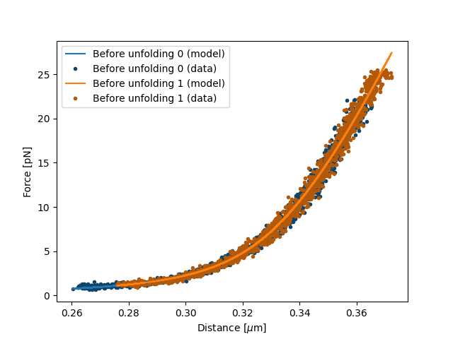
Let’s plot what we have fitted so far:
fit.fit()
plt.figure()
fit[model1].plot()
plt.xlabel(r"Distance [$\mu$m]")
plt.ylabel("Force [pN]")
plt.show()
Next, add data after unfolding to fit[model2]:
d_adk1 = file_adk1.fdcurves["adk5_curve1"].d["21s":"28s"].data
f_adk1 = file_adk1.fdcurves["adk5_curve1"].f["21s":"28s"].data

d_adk2 = file_adk2.fdcurves["adk5_curve2"]["20s":"28s"].d.data
f_adk2 = file_adk2.fdcurves["adk5_curve2"]["20s":"28s"].f.data

distances2 = [d_adk1[d_adk1 > 0], d_adk2[d_adk2 > 0]]
forces2 = [f_adk1[d_adk1 > 0], f_adk2[d_adk2 > 0]]

for i, (distance, force) in enumerate(zip(distances2, forces2)):
    fit[model2].add_data(f"After unfolding {i}", force, distance)
One thing to be careful about is that the we should not include points which are the result of an average between the folded and unfolded state. Next, we fit the data after the unfolding event. To speed up the computation, we fix the parameters that we already fitted:
>>> fit["DNA/Lc"].fixed = True
>>> fit["DNA/Lp"].fixed = True
>>> fit["DNA/St"].fixed = True
>>>
>>> fit["protein/Lp"].value = 0.7
>>> fit["protein/Lp"].lower_bound = 0.6
>>> fit["protein/Lp"].upper_bound = 1.0
>>> fit["protein/Lc"].value = 0.025
>>>
>>> fit.fit()
Fit
  - Model: DNA
  - Equation:
      f(d) = argmin[f](norm(DNA.Lc * (1 - (1/2)*sqrt(kT/(f*DNA.Lp)) + f/DNA.St)-d))

  - Data sets:
    - FitData(Before unfolding 0, N=1301)
    - FitData(Before unfolding 1, N=1301)
  - Model: inv(DNA_with_protein)
  - Equation:
      f(d) = argmin[f](norm(DNA.Lc * (1 - (1/2)*sqrt(kT/(d*DNA.Lp)) + d/DNA.St) + protein.Lc * (1 - (1/2)*sqrt(kT/(d*protein.Lp)) + d/protein.St)-d))

  - Data sets:
    - FitData(After unfolding 0, N=698)
    - FitData(After unfolding 1, N=799)

  - Fitted parameters:
    Name              Value  Unit      Fitted      Lower bound    Upper bound
    ----------  -----------  --------  --------  -------------  -------------
    DNA/Lp       19.75       [nm]      False           0.001              100
    DNA/Lc        0.349751   [micron]  False           0.00034            inf
    DNA/St      253.45       [pN]      False           1                  inf
    kT            4.11       [pN*nm]   False           3.77                 8
    protein/Lp    0.6        [nm]      True            0.6                  1
    protein/Lc    0.0216108  [micron]  True            0.00034            inf
    protein/St  250.87       [pN]      True            1                  inf
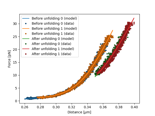
Now we have fitted both the data before and after unfolding. The results can be plotted as follows:
plt.figure()
fit[model1].plot()
fit[model2].plot()
plt.xlabel(r"Distance [$\mu$m]")
plt.ylabel("Force [pN]")
plt.show()
Accessing the model parameters for a specific data set is a little more complicated in this setting. If we want to obtain the parameters for “Before unfolding 1”, we’d have to invoke:
fit[model1]["Before unfolding 1"]