5. Image Stacks
Download this page as a Jupyter notebook
We can download the data needed for this tutorial directly from Zenodo using Pylake.
Since we don’t want it in our working folder, we’ll put it in a folder called "test_data":
filenames = lk.download_from_doi("10.5281/zenodo.7729700", "test_data")
Bluelake has the ability to export videos from different cameras as TIF files.
These videos can be opened using ImageStack:
stack = lk.ImageStack("test_data/stack.tiff") # Loading a stack.
Long videos are exported as a set of multiple files due to the size constraint on the TIF format.
In this case, you can supply the filenames consecutively (i.e. lk.ImageStack("tiff1.tiff", "tiff2.tiff"))
to treat them as a single object.
Full color RGB fluorescence images recorded with the widefield or TIRF functionality
are automatically reconstructed using the alignment matrices from Bluelake, if available. This functionality can be
turned off with the optional align keyword. Note that the align parameter has to be provided as a keyworded argument:
raw_stack = lk.ImageStack("test_data/stack.tiff", align=False)
5.1. Slicing and cropping
We can slice the stack by frame index:
stack_slice = stack[2:10] # Grab frame 3 to 9
or by time:
stack["2s":"10s"] # Slice from 2 to 10 seconds from beginning of the stack
You can also spatially crop to select a smaller region of interest:
# pixel coordinates as x_min, x_max, y_min, y_max
stack_roi = stack_slice.crop_by_pixels(10, 400, 10, 120)
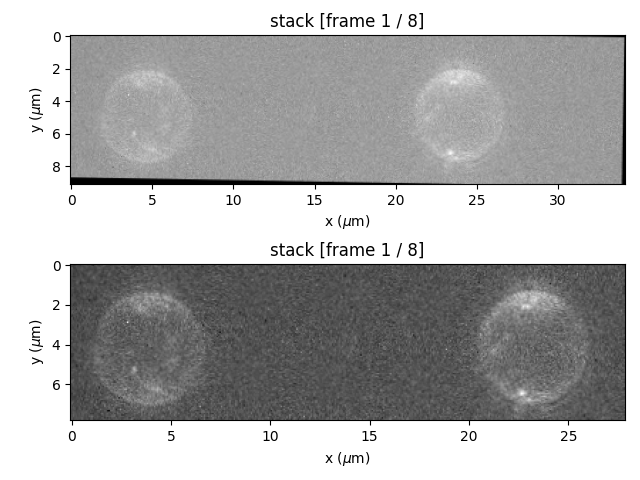
Cropping can be useful, for instance, after applying color alignment to RGB images since many
of the pixels near the edges don’t have data. We can see this by plotting just the "red" channel
(details of the plotting method are explained in the next section):
plt.figure()
plt.subplot(211)
stack_slice.plot("red")
plt.subplot(212)
stack_roi.plot("red")
plt.tight_layout()
plt.show()
Alternatively, you can crop directly by slicing the stack:
# slice with [frames, rows (y), columns (x)]
# equivalent to stack[2:10].crop_by_pixels(10, 400, 10, 120)
stack[2:10, 10:120, 10:400]
Here the first index can be used to select a subset of frames and the second and third indices
perform a cropping operation. Note how the axes are switched when compared to
crop_by_pixels() to follow the numpy
convention (rows and then columns).
You can also obtain the image stack data as a numpy array using the
get_image() method:
red_data = stack.get_image(channel="red") # shape = [n_frames, y_pixels, x_pixels]
rgb_data = stack.get_image(channel="rgb") # shape = [n_frames, y_pixels, x_pixels, 3 channels]
5.2. Plotting and exporting
Pylake provides a convenience plot() method to quickly
visualize your data. For details and examples see the Plotting Images section.
The stack can also be exported to TIFF format:
stack_roi.export_tiff("aligned_stack.tiff")
stack_roi[3:7].export_tiff("aligned_short_stack.tiff")  # export a slice of the ImageStack
Image stacks can also be exported to video formats. Exporting the red channel as a GIF can be done as follows:
stack_roi.export_video(
    "red",
    "test_red.gif",
    adjustment=lk.ColorAdjustment(20, 99, mode="percentile")
)
Or if we want to export a subset of frames (the first frame being 2, and the last frame being 7) of all three channels at a frame rate of 2 frames per second, we can do this:
stack_roi.export_video(
    "rgb",
    "test_rgb.gif",
    start_frame=2,
    stop_frame=7,
    fps=2,
    adjustment=lk.ColorAdjustment(20, 99, mode="percentile")
)
You can also export a video including correlated channel data by providing export_video() with a Slice:
file = lk.File("test_data/stack.h5")  # Loading a stack.
stack_roi.export_video(
    "rgb",
    "with_channel.gif",
    fps=2,
    adjustment=lk.ColorAdjustment(20, 99, mode="percentile"),
    channel_slice=file.force1x
)
Note
To export to an mp4 file, you will need to install ffmpeg. See Optional dependencies for more information.
5.3. Defining a tether
To define the location of the tether between beads, supply the (x, y) coordinates of the end points
to the define_tether() method:
stack_roi = stack[40:].crop_by_pixels(10, 400, 10, 120)
stack_tether = stack_roi.define_tether((6.94423, 4.22381), (20.47474,  4.08063))

plt.figure()
stack_tether.plot(
    "green",
    adjustment=lk.ColorAdjustment(0, 99, mode="percentile"),
    cmap=lk.colormaps.green,
)
stack_tether.plot_tether(lw=0.7)
plt.show()
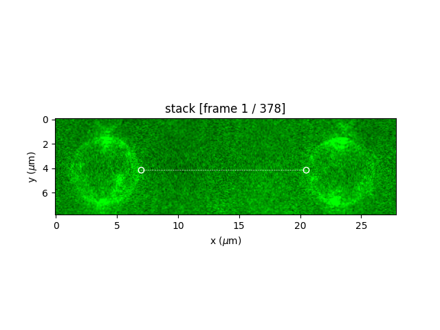
Note, after defining a tether location the image is rotated such that the tether is horizontal in
the field of view. You can also plot the overlay of the tether location using
plot_tether(**kwargs),
which also accepts keyword arguments that are passed to plt.plot().
You can also define a tether interactively using the crop_and_rotate() method. See the
Notebook widgets tutorial for more information.
5.4. Constructing a kymograph from an image stack
Once a tether is defined, the ImageStack can be converted to a Kymo using to_kymo():
plt.figure()
kymograph = stack_tether.to_kymo(half_window=5)
kymograph.plot(adjustment=lk.ColorAdjustment(1200, 2400))
plt.show()
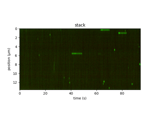
Here the argument half_window indicates how many additional pixels to average over on either side of the tether. The total number of lines averaged over is 2 * half_window + 1.
5.5. Correlating force with the image stack
Quite often, it is interesting to correlate events on the camera’s to channel data.
To quickly explore the correlation between images in a ImageStack and channel data
you can use the following function:
# Making a plot where force is correlated to images in the stack.
file = lk.File("test_data/stack.h5")  # Loading a stack.
stack[2:, 10:120, 10:400].plot_correlated(
    file.force1x,
    channel="rgb",
    frame=208,
    adjustment=lk.ColorAdjustment(20, [98, 99.9, 100], mode="percentile")
)
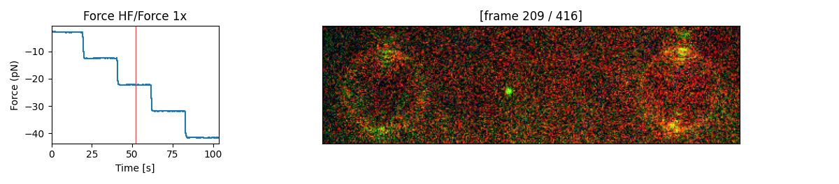
If the plot is interactive (for example, when %matplotlib widget is used in a Jupyter notebook), you can click
on the left graph to select a particular force. The corresponding video frame will then automatically appear on the right.
In some cases, additional processing may be needed, and we wish to have the data
downsampled over the video frames. This can be done using the downsampled_over()
method with timestamps obtained from the ImageStack:
# Determine the force trace averaged over frame 2...9.
file.force1x.downsampled_over(stack[2:10].frame_timestamp_ranges())
By default, this averages only over the exposure time of the images in the stack.
If you wish to average over the full time range from the start of the scan to the next scan, pass the extra parameter include_dead_time=True:
file.force1x.downsampled_over(stack[2:10].frame_timestamp_ranges(include_dead_time=True))