9. Kymotracking
Download this page as a Jupyter notebook
Note
This tutorial describes the programmatic use of various tracking algorithms and downstream analyses. Since the tracking algorithms have many input parameters that must be tweaked for each kymograph or region of interest, it is generally easier to use the interactive widget provided by Pylake. See the Notebook widgets tutorial for more information.
Kymographs are a vital tool in understanding binding events on DNA. These are generated by acquiring one-dimensional scans along the DNA tether over time. Bound particles are seen as tracks of signal along the time axis. The spatial dimension tells us information about the movement of the particle along the DNA tether. For instance, statically bound particles appear as horizontal tracks, while particles moving directed in a particular orientation appear as diagonal tracks in the kymograph.
Determining the spatial and temporal coordinates of these particles is the first step in various types of analysis, discussed below. Pylake comes with a few features that enable you to do so.
Kymotracking is usually performed in two steps: an image processing step, followed by a tracking step, where the actual coordinates of bound particles are found. Let’s take a look at one particular implementation, the greedy algorithm.
We can download the data needed for this tutorial directly from Zenodo using Pylake.
Since we don’t want it in our working folder, we’ll put it in a folder called "test_data":
filenames = lk.download_from_doi("10.5281/zenodo.7729525", "test_data")
9.1. Using the greedy algorithm
First, we need to get a kymograph to perform the tracking on. Let’s grab a kymograph from a Bluelake file and see what it looks like with the correlated force data:
# define a color adjustment so we can see the data better
adjustment = lk.ColorAdjustment(0, 99.5, mode="percentile")

file = lk.File("test_data/kymo.h5")
name, kymo = file.kymos.popitem()

kymo.plot_with_force("1x", "rgb", adjustment=adjustment, aspect_ratio=0.5)
plt.show()
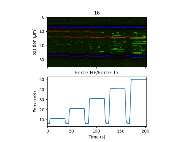
This experiment shows stochastic binding of a fluorescently labeled protein to a DNA tether at various forces. We also see the bead edges in this kymograph as dark bands (the absence of background fluorescence from the bulk solution).
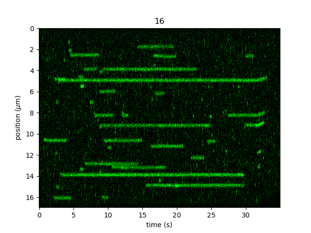
Let’s only take a subsection of the kymograph at 40 pN and without the beads to make sure that we don’t get any spurious track detections
from the bead edges. We’ll store this as a new Kymo instance and see what it looks like:
kymo40 = kymo["127s":"162s"]
kymo40 = kymo40.crop_by_distance(9, 26)

plt.figure()
kymo40.plot("green", aspect="auto", adjustment=adjustment)
plt.show()
Running the algorithm is easy using the function track_greedy():
tracks = lk.track_greedy(kymo40, "green")
The result is a KymoTrackGroup:
print(type(tracks))  # <class 'lumicks.pylake.kymotracker.kymotrack.KymoTrackGroup'>
print(len(tracks))  # 134
This is a custom list of KymoTrack objects. We can access the individual tracks by indexing just
like an ordinary list:
track = tracks[0]

print(type(track))  # <class 'lumicks.pylake.kymotracker.kymotrack.KymoTrack'>
print(len(track))  # 1
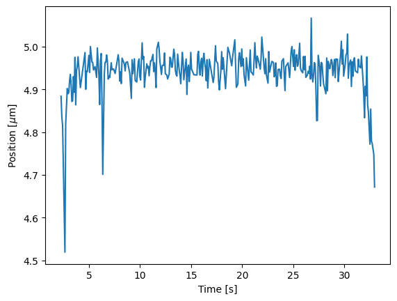
We can access the determined time and positions of each track from the seconds and
position properties. For instance, if we want to plot the coordinates
of the longest track we can do:
longest_track_idx = np.argmax([len(track) for track in tracks])  # Get the index of the longest track
longest_track = tracks[longest_track_idx]

plt.figure()
plt.plot(longest_track.seconds, longest_track.position)
plt.xlabel("Time [s]")
plt.ylabel(r"Position [$\mu$m]")
plt.show()
We can access an estimate for the photon counts contributing to the track in photon_counts:
plt.figure()
plt.plot(longest_track.seconds, longest_track.photon_counts)
plt.xlabel('Time [s]')
plt.ylabel('Photon counts [#]')
plt.show()
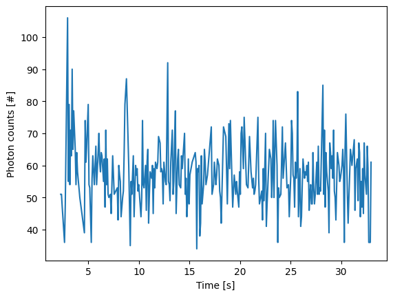
By default, this estimate is based on summing the photon counts of an odd number of pixels around the peak position.
As such, it will include a contribution from any background signal that may be present.
The number of pixels to sum is set by the tracking parameter track_width.
More accurate estimates of the photons emitted by a particle can be obtained using gaussian refinement detailed further below.
Sometimes, we can have very short spurious tracks. To remove these we can use filter_tracks().
For example, to omit all tracks with fewer than 4 detected points, we can invoke:
print(len(tracks))  # the number of tracks originally detected -- 134

tracks = lk.filter_tracks(tracks, minimum_length=4)
print(len(tracks))  # the number of tracks after filtering -- 35
We can also filter by track duration.
>>> print(len(lk.filter_tracks(tracks, minimum_duration=1)))
26
There are also convenience plotting functions for both KymoTrack.plot()
and KymoTrackGroup.plot(). We can see the detected tracks overlaid
on the kymograph with just 2 lines of code:
plt.figure()
kymo40.plot(channel="green", aspect="auto", adjustment=adjustment)
tracks.plot()
plt.show()
We can improve the tracking results by adjusting a number of tracking parameters. For instace, we can inspect a track to estimate the spatial width
and signal level by zooming in and adding a little color legend using plt.colorbar() (if you’re using an
interactive backend you can also hover over a pixel in the image to inspect it’s value):
plt.figure()
# to show the color bar, we need the plotted image handle from the plot method
image = kymo40.plot("green", aspect="auto", adjustment=adjustment, interpolation="none")
plt.xlim(7.5, 25.5)
plt.ylim(8.8, 9.8)
plt.colorbar(image)
plt.show()
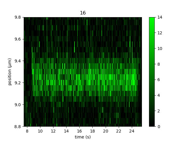
We can see the tracks are about 0.3 microns wide and the signal level is around 10-14 counts. We can use this information when tracking
by setting the track_width and pixel_threshold parameters, respectively. Larger values for track_width reject more noise, but at the cost of
potentially merging tracks that are close together. We also see that sometimes a particle momentarily disappears or drops below
the pixel_threshold, due to blinking for instance. To still connect these in a single track, we want to allow for some gaps in the connection step.
We can set this with the window parameter; let’s use a window size of 6 pixels in this test:
custom_tracks = lk.track_greedy(kymo40, "green", track_width=0.3, pixel_threshold=10, window=6)
custom_tracks = lk.filter_tracks(custom_tracks, minimum_length=4)
print(len(custom_tracks))  # 41

plt.figure()
kymo40.plot("green", aspect="auto", adjustment=adjustment)
custom_tracks.plot()
plt.show()
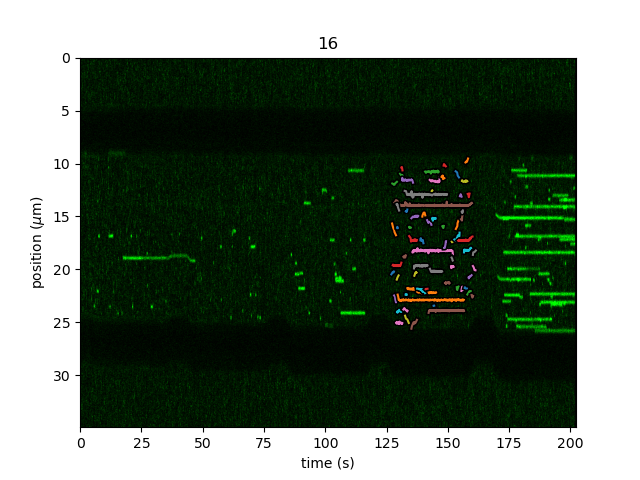
Sometimes we want to track only part of a kymograph without manually slicing and cropping. We can do this by passing the rect argument to
track_greedy(), which defines a rectangle over which to track peaks. The coordinates of this parameter are of the form
[[min_time, min_position], [max_time, max_position]]. To track the same region as before, we can do:
tracks = lk.track_greedy(kymo, "green", rect=[[127, 9], [162, 26]])
tracks = lk.filter_tracks(tracks, minimum_length=4)

plt.figure()
kymo.plot("green", aspect="auto", adjustment=adjustment)
tracks.plot()
plt.show()
9.2. Localization refinement
9.2.1. Centroid
Once we are happy with the tracks found by the algorithm, we may still want to refine them. Since the algorithm finds
tracks by determining local peaks and stringing these together, it is possible that some scan lines in the kymograph
don’t have an explicit point on the track associated with them. Using refine_tracks_centroid() we
can refine the tracks found by the algorithm. This function interpolates the tracks such that each time point gets its
own point on the track. Subsequently, these points are then refined using a brightness weighted centroid.
Brightness weighted centroid refinement can suffer from a bias when there is background signal. This bias artificially
pulls the localization towards the center of the pixel. By default, Pylake applies a correction for this based on [BMML08].
You can turn this off by using bias_correction=False with track_greedy() and refine_tracks_centroid().
Let’s perform track refinement with two different values for track_width to see the effect:
# re-track our kymo
tracks = lk.track_greedy(kymo40, "green", track_width=0.3)
tracks = lk.filter_tracks(tracks, minimum_length=4)

# refine with the same track_width
refined = lk.refine_tracks_centroid(tracks, track_width=0.3)
# refine with double the track_width
refined_wider = lk.refine_tracks_centroid(tracks, track_width=0.6)

plt.figure()
kymo40.plot("green", aspect='auto', interpolation="none", cmap="bone")
tracks[12].plot(marker="o", show_outline=False, label="track, track width = 0.3", c="white")
refined[12].plot(marker="o", mfc="none", show_outline=False, label="refined, track width = 0.3", c="tab:orange")
refined_wider[12].plot(marker="o", mfc="none", show_outline=False, label="refined, track width = 0.6", c="tab:olive")

plt.xlim(8.5, 10.5)
plt.ylim(8.8, 9.8)
plt.legend()
plt.tight_layout()
plt.show()
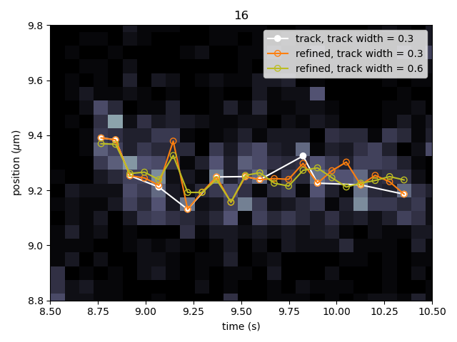
We can see that a few points were added post refinement (shown in orange). Increasing the track_width (shown in green) takes into account
more pixels in the vertical direction during refinement. While the result is not significantly different, problems will occur if tracks are
close together.
9.2.2. Maximum Likelihood Estimation
While centroid refinement is fast, its results can be inaccurate in cases of high background or lines that are very close together. In such cases,
it is better to rely on a different refinement method. One alternative is to use Maximum Likelihood Estimation (MLE). This method is available
through the function refine_tracks_gaussian(). Gaussian refinement assumes that the point spread function follows a Gaussian shape
and the photon counts are Poisson distributed. It also includes an offset to model the background counts (adapted for 1D data from [MCSF10]).
For each frame in the kymograph, we fit a small region around the tracked peak to the data by maximizing the following likelihood function:
where \(\theta\) represents the parameters to be fitted, \(M\) is the number of pixels and \(n_i\) and \(E_i(\theta)\) are the observed photon count and expectation value for pixel \(i\). The shape of the peak is described with a Gaussian expectation function
Here \(N\) is the total photons emitted in the fitted image (scan line), \(a\) is the pixel size, \(\mu\) is the peak center, \(x_i\) is the pixel center position, \(\sigma^2\) is the variance, and \(b\) is the background level in photons/pixel.
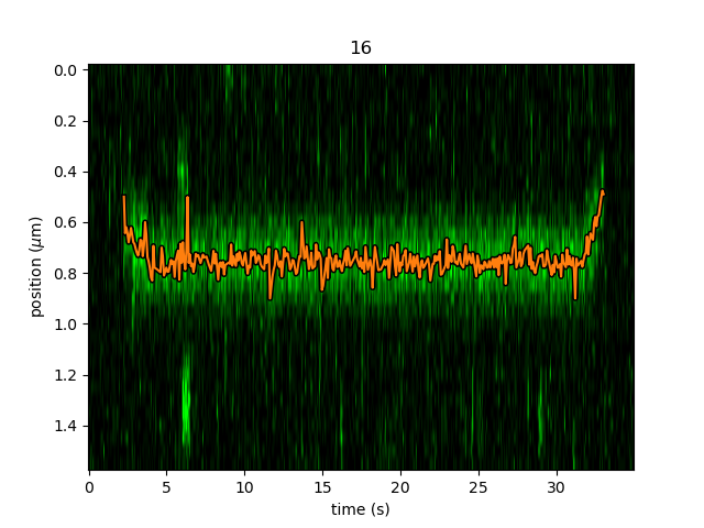
This function is called in a similar manner as the centroid refinement. Since the MLE optimization is significantly slower than the centroid method, let’s refine just a single long track:
# track a subsection of the kymo
cropped_kymo = kymo40.crop_by_distance(4.2, 5.8)
tracks = lk.track_greedy(cropped_kymo, "green", track_width=0.3, window=10, pixel_threshold=9)
tracks = lk.filter_tracks(tracks, minimum_length=10)
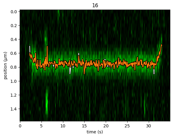
# perform the gaussian refinement
refined = lk.refine_tracks_gaussian(tracks, window=3, refine_missing_frames=False, overlap_strategy="skip")
plt.figure()
cropped_kymo.plot("green", adjustment=adjustment, aspect="auto")
refined.plot()
plt.show()
While centroid refinement provides a simple sum of the surrounding pixels, Gaussian refinement determines the integrated area of the peak as one of the fitting parameters.
It also explicitly takes into account background signal that may be present.
This means that if the fit is good, Gaussian refinement should provide a more accurate estimate of the photon counts originating from the fluorophore.
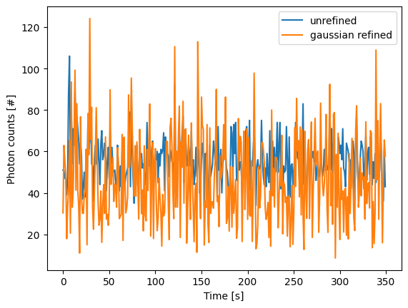
KymoTrack instances returned from the refinement function have updated photon_counts based on the optimized integrated peak area:
plt.figure()
for unrefined_track, refined_track in zip(tracks, refined):
    plt.plot(unrefined_track.photon_counts, label="unrefined")
    plt.plot(refined_track.photon_counts, label="gaussian refined")

plt.xlabel('Time [s]')
plt.ylabel('Photon counts [#]')
plt.legend()
plt.show()
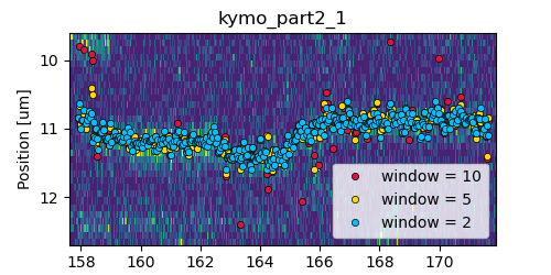
The number of pixels to be included in the fit is determined by the window argument, with a total size of 2*window+1 pixels.
The exact value of this parameter is dependent on the quality of the data and should be balanced between including enough pixels to fully
capture the peak lineshape while avoiding overlap with other traces or spurious high-photon count pixels due to noise or background.
The effect of different window sizes are demonstrated in the following figure:
As noted in the above section, there may be intermediate frames which were not detected in the original track. We can optionally interpolate
an initial guess for these frames before the Gaussian refinement by setting the argument
refine_missing_frames=True. It should be noted, however, that frames with low photons counts (for instance due to fluorophore blinking)
may not be well fit by this algorithm.
Additionally, the presence of a nearby track wherein the sampled pixels of the two tracks overlap may interfere with the
refinement algorithm. How the algorithm handles this situation is determined by the overlap_strategy argument.
Setting overlap_strategy="ignore" simply ignores nearby tracks and fits the data. In this case, the resulting localization will be biased
as signal from the nearby track will “pull” the location parameter towards it.
A problem with the refinement in this case will manifest as the peak of the second track is found rather than that of the current track.
Sometimes this can be avoided by decreasing the size of the window argument such that overlap no longer occurs.
A better alternative is to use overlap_strategy="simultaneous".
When this option is specified, peaks where the windows overlap are fitted simultaneously (using a shared offset parameter).
Alternatively, we can simply ignore these frames by using overlap_strategy="skip", in which case these frames are simply dropped from the track.
There is also an optional keyword argument initial_sigma that can be used to pass an initial guess for \(\sigma\)
in the above expectation equation to the optimizer. The default value is 1.1 * pixel_size.
When tracks are well separated, it is possible to use a relatively large window and estimate the peak parameters and offset from the fit directly. When this is not the case, one can estimate the offset separately. To do this, crop an area of the kymograph that only has background in it. Computing the appropriate photons/pixel background considering a Poissonian noise model can be done by computing the mean of the pixels in this area. Here we crop the original kymograph from 25 to 27 seconds and 10 to 12 microns:
background_kymo = kymo["25s":"27s"]
background_kymo = background_kymo.crop_by_distance(10, 12)
offset = np.mean(background_kymo.get_image("green"))
print(offset)
The independently determined offset (in photons per pixel) can then be provided directly to
lk.refine_tracks_gaussian:
refined_with_offset = lk.refine_tracks_gaussian(tracks, window=3, refine_missing_frames=False, overlap_strategy="skip", fixed_background=offset)

plt.figure()
cropped_kymo.plot("green", adjustment=adjustment, aspect="auto")
refined.plot(c="w")
refined_with_offset.plot(c="tab:orange")
plt.show()
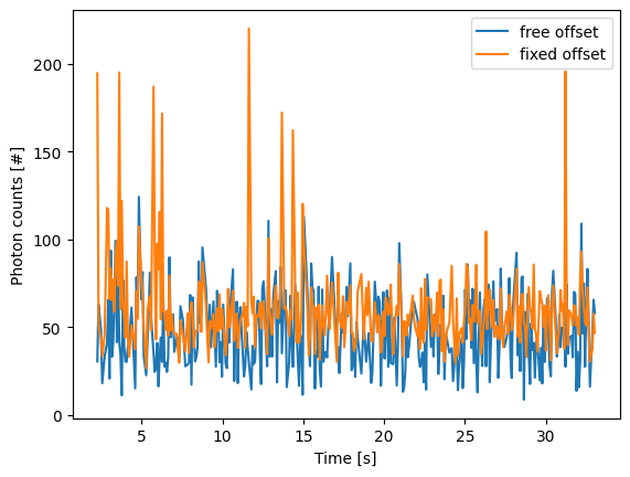
In this case the parameter will not be fitted, but fixed to the user specified value. This can help reduce the variance of the parameter estimates. Estimating an offset independently prior to fitting can improve the precision of the estimates (since it requires fewer parameters to be estimated for each window):
plt.figure()
for free_offset, fixed_offset in zip(refined, refined_with_offset):
    plt.plot(free_offset.seconds, free_offset.photon_counts, label="free offset")
    plt.plot(fixed_offset.seconds, fixed_offset.photon_counts, label="fixed offset")

plt.xlabel('Time [s]')
plt.ylabel('Photon counts [#]')
plt.legend()
plt.show()
Note that this method should only be used if the background can be assumed to be constant over time and position.
9.3. Using the lines algorithm
The second algorithm present is an algorithm that works purely on signal derivative information. It works by blurring the image, and then performing sub-pixel accurate line detection. It can be a bit more robust to low signal levels, but is generally less temporally and spatially accurate due to the blurring involved:
tracked_lines = lk.track_lines(kymo40, "green", line_width=0.3, max_lines=50)
The interface is mostly the same, aside from an extra required parameter named max_lines which indicates the maximum
number of lines we want to detect.
9.4. Extracting summed intensities
Sometimes, it can be desirable to extract pixel intensities in a region around our kymograph track.
We can quite easily extract these using the method sample_from_image().
Warning
Prior to version 1.1.0 the method sample_from_image() had a bug that assumed the
origin of a pixel to be at the edge rather than the center of the pixel.
Consequently, the sampled window could frequently be off by one pixel.
The old (incorrect) behavior is maintained until the next major release (version 2.0) to ensure backward
compatibility. It is recommended to include the argument correct_origin=True which results in using the correct origin.
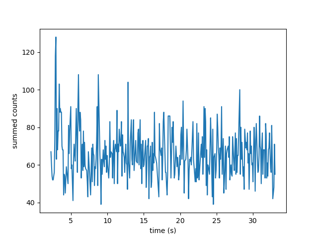
If we want to sum the pixels in a 11 pixel area around the longest kymograph track, we can invoke:
longest_track_idx = np.argmax([len(track) for track in tracks])
longest_track = tracks[longest_track_idx]

plt.figure()
plt.plot(longest_track.seconds, longest_track.sample_from_image(num_pixels=5, correct_origin=True))
plt.xlabel('time (s)')
plt.ylabel('summed counts')
plt.show()
Here num_pixels is the number of pixels to sum on either side of the track.
Note
For tracks obtained from tracking or refine_tracks_centroid(), the photon counts found in the attribute photon_counts are computed by sample_from_image() using num_pixels=np.ceil(track_width / pixelsize) // 2 where track_width is the track width used for tracking or refinement.
9.5. Averaging channel data over tracks
It is also possible to average channel data over the track using sample_from_channel().
For example, let’s find out what the force was during a particular track:
force_slice = file.force1x
track_force = longest_track.sample_from_channel(force_slice, include_dead_time=True)
When you call this function with a Slice, it returns another Slice with the downsampled channel data.
For every point on the track, the corresponding kymograph scan line is looked up and the channel data is averaged over the entire duration of that scan line.
The parameter include_dead_time specifies whether the dead time (the time it takes the mirror to return to its initial position after each scan line) should be included in this average.
For tracks which have not been refined (see Localization refinement) the result from this function may skip some scan lines entirely.
We can plot these slices just like any other. Plotting this slice, we can see that the protein detaches shortly after the force drops:
plt.figure()
force_slice.plot(label="force (whole file)")
track_force.plot(start=force_slice.start, marker=".", label="force (longest track)")
plt.legend(loc="upper left")
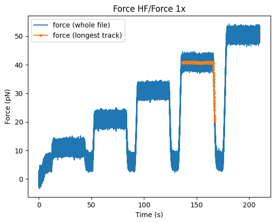
We plotted the track here putting the time zero at the start time of the entire force plot by passing its start time.
9.6. Plotting binding histograms
We can easily plot some histograms of the binding events located with the kymotracker with
plot_binding_histogram():
# re-track so we have fresh data to work with
tracks = lk.track_greedy(kymo40, "green", track_width=0.3)
tracks = lk.filter_tracks(tracks, minimum_length=4)
tracks = lk.refine_tracks_centroid(tracks, track_width=0.3)

plt.figure()
tracks.plot_binding_histogram(kind="binding")
plt.show()
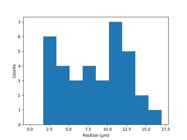
The kind argument controls what we want to plot. Here kind="binding" indicates that we only wish to analyze
the initial binding events (the first position of each track). We can also use kind="all" to include all of the
bound positions for each track.
We can optionally supply a bins argument, which is forwarded to np.histogram().
For instance, we can increase the number of bins from 10 (the default) to 30:
plt.figure()
tracks.plot_binding_histogram("binding", bins=30)
plt.show()
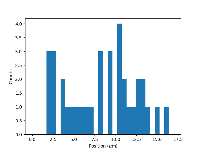
When an integer is supplied to the bins argument, the full position range of the kymograph is used to calculate
the bin edges (this is equivalent to using np.histogram(data, bins=n, range=(0,
max_position))). This facilitates comparison of histograms calculated from
different kymographs, as the absolute x-scale is dependent on the kymograph acquisition options,
rather than the positions of the tracks.
Alternatively, it is possible to supply a custom array of bin edges:
plt.figure()
tracks.plot_binding_histogram(kind="all", bins=np.linspace(12, 18, 75), fc="#dcdcdc", ec="tab:blue")
plt.show()
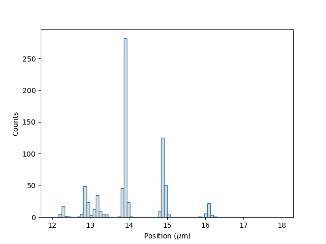
This snippet also demonstrates how we can pass keyword arguments (forwarded to plt.bar()) to format the histogram.
9.7. Importing and exporting kymograph tracks
We can export the coordinates of the tracks to a csv file using the save()
method with the desired file name:
tracks.save("tracks.csv")
We can include photon counts (calculated with sample_from_image())
by passing a width in pixels to sum counts over:
tracks.save("tracks_signal.csv", sampling_width=3, correct_origin=True)
We can re-import these tracks into Pylake at a later time using the load_tracks() function:
tracks = lk.load_tracks("tracks.csv", kymo40, "green")
Note
The kymo and channel arguments provided must be the same as the ones used to generate the tracks.
This includes any processing (e.g. cropping, downsampling, flipping, etc.) that was performed on the kymograph.
9.8. How the algorithms work
9.8.1. track_greedy
The first method track_greedy() implemented for performing such a tracking is based on [MPP16, SK05].
It starts by performing peak detection, performing a grey dilation on the image, and detection which pixels remain
unchanged. Peaks that fall below a certain intensity threshold are discarded. Since this peak detection operates at a
pixel granularity, it is followed up by a refinement step to attain subpixel accuracy. This refinement is performed by
computing an offset from a brightness-weighted centroid in a small neighborhood w around the pixel.
Where m is given by:
After peak detection the feature points are linked together using a forward search analogous to [MPP16]. This is in contrast with the linking algorithm in [SK05] which uses a graph-based optimization approach. This linking step traverses the kymograph, tracking particles starting from each frame.
The algorithm starts at time frame one (the first pixel column).
It selects the peak with the highest pixel intensity and initiates the first track.
Next, it evaluates the subsequent frame, and computes a connection score for each peak in the next frame (to be specified in more detail later).
If a peak is found with an acceptable score, the peak is added to the track.
When no more candidates are available we look in the next
windowframes to see if we can find an acceptable peak there, following the same procedure.Once no more candidates are found in the next
windowframes, the track is terminated and we proceed by initiating a new track from the peak which is now the highest.Once there are no more peaks in the frame from which we are currently initiating tracks, we start initiating tracks from the next frame. This process is continued until there are no more peaks left to trace.
The score function is based on a prediction of where we expect future peaks. Based on the peak location of the tip of
the track x and a velocity v, it computes a predicted position over time. The score function assumes a Gaussian
uncertainty around that prediction, placing the mean of that uncertainty on the predicted extrapolation. The width of
this uncertainty is given by a base width (provided as sigma) and a growing uncertainty over time given by a diffusion
rate. This results in the following model for the connection score.
Here N refers to a normal distribution. In addition to the model, we also have to set a cutoff, after which we deem
peaks to be so unlikely to be connected that they shouldn’t be. By default, this cutoff is set at two sigma. Scores
outside this cutoff are set to zero which means they will not be accepted as a new point.
9.8.2. track_lines
The second algorithm track_lines() is an algorithm that looks for curvilinear structures in an image. This method is based on sections
1, 2 and 3 from [Ste98]. This method attempts to find lines purely based on the derivatives of the
image. It blurs the image based with a user specified line width and then attempts to find curvilinear sections.
Based on the second derivatives of the blurred image, a Hessian matrix is constructed. This Hessian matrix is decomposed using an eigenvector decomposition to obtain the perpendicular and tangent directions to the line. To attain subpixel accuracy, the maximum is computed perpendicular to the line using a local Taylor expansion. This expansion provides an offset on the pixel position. When this offset falls within the pixel, then this point is considered to be part of a line. If it falls outside the pixel, then it is not a line.
This provides a narrow mask, which can be traced. Whenever ambiguity arises on which point to connect next, a score comprised of the distance to the next subpixel minimum and angle between the successive normal vectors is computed. The candidate with the lowest score is then selected.
Since this algorithm is specifically looking for curvilinear structures, it can have issues with structures that are more blob-like (such as short-lived fluorescent events) or diffusive traces, where the particle moves randomly rather than in a uniform direction.
9.9. Studying diffusion processes
Pylake supports a number of methods for studying diffusive processes.
These methods rely on quantifying how much the particle moves between each frame of the kymograph.
Ideally, tracked lines with many gaps in their tracking (due to the threshold not being met) should be refined using refine_tracks_centroid() prior to diffusive analysis.
Regions without signal (such as when the fluorophore blinks) should not be tracked, since they can bias the results because the positions cannot reliably be estimated.
9.9.1. Covariance-based estimator
If the diffusive motion is clearly visible, then a generally robust and unbiased method method for computing the free diffusion is the covariance-based estimator (CVE) [Ves16, VBF14].
It bases its estimate of the diffusion constant on the change in the particle position between observations.
This method should generally be your first choice when trying to estimate diffusion constants from tracks.
It is the easiest method to use (no parameters) and it can handle unequal length tracks and tracks which have untracked gaps due to blinking.
To estimate the diffusion constant using the CVE for a single track, you can simply call estimate_diffusion() while passing "cve" as method:
diffusion_estimate = tracks[0].estimate_diffusion(method="cve")
The results are provided as a DiffusionEstimate which contains the requested estimates and some metadata.
You can call the same estimation function on a KymoTrackGroup which will give you a list containing estimates for each track in the group.
If all the tracks in a group are expected to have the same diffusion constant, then the best estimate can be obtained by weighting the estimates for the individual tracks by the number of points contributing to each estimate.
Pylake provides a convenience function for obtaining such estimates at the group level ensemble_diffusion():
tracks.ensemble_diffusion(method="cve")
If it is safe to assume that the localization variance is the same for all the tracks, then one can achieve a more precise estimate for individual tracks by estimating this quantity at an ensemble level and then using that in the per-track estimation procedure:
ensemble_estimate = tracks.ensemble_diffusion("cve")
print(ensemble_estimate)

# Pass the ensemble localization uncertainties to the method
per_track_estimate = tracks.estimate_diffusion(
    "cve",
    localization_variance=ensemble_estimate.localization_variance,
    variance_of_localization_variance=ensemble_estimate.variance_of_localization_variance
)
print(per_track_estimate[0])
For more information on this procedure and how it affects the estimation uncertainties, please refer to the theory section on diffusive motion.
9.9.2. Mean Squared Displacements
Mean Squared Displacements (MSD) are a different quantity used to characterize particle motion.
Purely diffusive processes leads to Mean Squared Displacements that linearly depend on the lag time (the time between two data points for which the displacement is calculated. Note this is not the same as the scan line time).
MSDs for individual tracks are available through msd():
msd = tracks[0].msd()
which returns a tuple of lags and MSD estimates. If we only wish MSDs up to a certain lag, we can provide a max_lag argument:
>>> tracks[0].msd(max_lag=5)
(array([0.16, 0.32, 0.48, 0.64, 0.8 ]), array([ 3.63439512,  6.13181603,  9.08823918, 11.43574189, 12.61152129]))
If it is safe to assume that all particles exhibit the same diffusive motion, one can calculate the ensemble and time-averaged MSD for an entire group of tracks using the method ensemble_msd():
ensemble_msd = tracks.ensemble_msd()
This returns a EnsembleMSD class which contains the requested estimates
along with some metadata and a plot() method. Because this particular
protein is not diffusive, plotting this data is of little value; however, see the additional discussion in the
theory section for diffusive processes.
One thing that is important to note is that the MSDs of one track for different lags are highly correlated and that estimates at larger lags are far less reliable. Therefore one should not fit these values as though they were independent data points. Doing so leads to very imprecise estimates.
9.9.3. Ordinary Least Squares
Considering that the MSDs follow a linear curve for pure diffusion, it makes sense to fit a linear curve to these estimates.
We can do this using Ordinary Least Squares (OLS), which performs an unweighted fit of the data.
In Pylake, you can obtain OLS estimates for a KymoTrack using:
>>> tracks[0].estimate_diffusion(method="ols")
DiffusionEstimate(value=7.804440367653842, std_err=2.527045387449447, num_lags=2, num_points=80, method='ols', unit='um^2 / s')
This method performs a linear regression on the estimated MSD values.
Fitting an appropriate number of lags given the observational noise is crucial for getting a good estimate with this method.
By default, this method will determine the optimal number of lags to use in the fit as specified in [MB12].
You can however, override this optimal number of lags, by specifying a max_lag parameter.
Warning
It is not recommended to apply Ordinary Least Squares to invididual tracks if they are very short since it will produce biased results in such scenarios. Care must also be taken when averaging results from multiple tracks to obtain a mean diffusion coefficient. While the estimated number of lags may be optimal for analyzing an individual track, averaging the results from tracks with different number of lags can lead to a biased estimate. For more information on this, see the theory section for diffusive processes.
The uncertainty estimate and optimal number of lags obtained for Ordinary Least Squares relies on having a successful positional localization for every frame in a KymoTrack.
If frames are missing, then this method will issue a warning with the suggestion to refine tracks prior to estimation using Localization refinement. If this is not possible, please switch to Covariance-based estimator.
If the diffusion constant can be assumed the same for an ensemble of tracks, it is possible to get a more precise estimate of the diffusion constant by first calculating the MSD for all of them, and then performing only a single fit.
You can do this with Pylake by using ensemble_diffusion():
tracks.ensemble_diffusion(method="ols")
For more information on this procedure and its performance, please refer to the theory section.
9.9.4. Generalized Least Squares
Generalized linear least squares suffers less from including more lags than are optimal as it takes into account the covariance matrix of the MSD [BvBulowH20].
This method is slower, since it has to solve some implicit equations. In addition to that, its current implementation cannot cope with missing frames.
It can be selected by choosing "gls" for the method:
tracks.estimate_diffusion(method="gls", max_lag=30)
Note that while the choice of number of lags to include is less critical, it is still a good idea to make sure not to include MSD values where very little averaging has taken place. Pylake does not offer an ensemble averaged variant of the generalized least squares estimator.
Note
The Generalized Least Squares method for estimating the diffusion constant relies on having a successful positional localization for every frame in a KymoTrack.
If frames are missing, then this method will raise an exception with the suggestion to refine tracks prior to estimation using Localization refinement. If this is not possible, please switch to Covariance-based estimator.
9.10. Dwelltime analysis
The lifetime of the bound state(s) can be determined using fit_binding_times(). This method defines
the bound dwelltime as the length of each track in seconds.
Note
Tracks which start in the first frame of the kymograph or end in the last frame are excluded from the analysis. This is because, such tracks have
ambiguous binding times as the start or end of the track is not known definitively. If these tracks were included in the analysis, this could lead to minor
biases in the results, especially if the number of tracks that meet this criterion is large relative to the total number.
This behavior can be overridden with the keyword argument exclude_ambiguous_dwells=False.
To fit the bound dwelltime distribution to a single exponential (the simplest case) simply call:
dwell = tracks.fit_binding_times(n_components=1, observed_minimum=False, discrete_model=True)
This returns a DwelltimeModel object which contains information about the optimized model, such as the lifetime of the state in seconds:
print(dwell.lifetimes)
Note
The flag discrete_model=True takes into account that the binding times are discretized to multiples of the kymograph line time.
This is a more accurate model for the data and leads to smaller biases when estimating.
Starting from Pylake 2.0.0 this will become the new default.
Note
The min_observation_time and max_observation_time arguments to the underlying DwelltimeModel are set automatically by this method.
The minimum length of the tracks depends not only on the kymograph line scan time but also the specific input parameters used for the tracking algorithm.
In earlier versions, Pylake used the shortest track time and the length of the experiment, respectively.
Starting in Pylake 1.2.0, it is possible to use the minimum possible dwell time calculated from the tracking and acquisition parameters by specifying observed_minimum=False.
This is the preferable method, since the former can lead to biases for kymographs with few events.
In the next major version of Pylake (2.0.0) this flag will become the default.
We can also try a double exponential fit:
dwell2 = tracks.fit_binding_times(n_components=2, observed_minimum=False, discrete_model=True)
print(dwell2.lifetimes)  # list of bound lifetimes
print(dwell2.amplitudes)  # list of fractional amplitudes for each component
For a detailed description of the optimization method and available attributes/methods see the Dwelltime Analysis section in Population Dynamics.
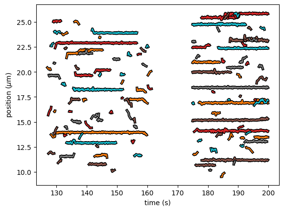
9.11. Global analysis
Sometimes, we want to combine tracking results from multiple Kymographs to determine biophysical parameters with increased precision.
We can do this, by simply adding KymoTrackGroup instances together.
We’ll demonstrate this functionality using multiple sections on a single Kymo, but it generalizes to tracks from different kymographs:
tracks1 = lk.filter_tracks(lk.track_greedy(kymo, "green", rect=[[127, 9], [162, 26]]), minimum_length=4)
tracks2 = lk.filter_tracks(lk.track_greedy(kymo, "green", rect=[[175, 9], [200, 26]]), minimum_length=4)

multiple_groups = tracks1 + tracks2
multiple_groups.plot()
The API for the different methods is identical, requiring no changes to your downstream analysis compared to the case of tracks from a single kymograph. For instance, one can compute the binding lifetime with:
multi_dwell = multiple_groups.fit_binding_times(n_components=2, observed_minimum=False, discrete_model=True)
print(multi_dwell.lifetimes)  # list of bound lifetimes
print(multi_dwell.amplitudes)  # list of fractional amplitudes for each component
Warning
When working with KymoTrackGroup instances tracked from different kymographs, certain features require that all source kymographs have the same pixel size and scan line times (e.g., ensemble_msd() and ensemble_diffusion("ols")).
Such methods will raise an exception if these conditions are not met.