Diffusion analysis

Download this page as a Jupyter notebook

Pylake supports a number of methods for studying diffusive processes. These methods rely on quantifying the movement of the fluorophore. This section details some of the available methods and details some pitfalls with each of them. In this chapter, we will be making use of simulated data, so that we can study the quality of our estimates while knowing the ground truth. Note that the code to perform these simulation is included, so that you can play with them and produce similar graphs which are more tailored to your own experimental conditions. For more information on tracking the particles in a kymograph, refer to Kymotracking and specifically the section on diffusion regarding diffusion analysis on kymographs.

Simulating 1D free diffusion

The displacements of a particle undergoing free diffusion are uncorrelated over time and distributed according to a normal distribution. The standard deviation of this distribution follows from the diffusion equation and is given by: \(\sqrt{2 D \Delta t}\). We can simulate 1D diffusion as:

\[x_{i+1} = x_i + \sqrt{2 D \Delta t} \mathcal{N}(0, 1)\]

Here \(x_i\) is the coordinate at time frame \(i\), \(D\) is the diffusion constant, \(\Delta t\) is the time step and \(\mathcal{N}(0, 1)\) is a sample from a normal distribution with a mean of zero and a standard deviation of 1. Our observations of the particle’s position are subject to noise. In this section, we model this as Gaussian additive noise on the positions in the track.

Note that free diffusion assumes that the space available for diffusion \(L\) is sufficiently large that the measurement time interval is much smaller than \(L / 2D\) [QSE91]:

To simulate diffusive tracks with observation noise, we can use simulate_diffusive_tracks():

tracks = lk.simulation.simulate_diffusive_tracks(diffusion_constant=1.0, steps=40, dt=0.01, observation_noise=0.1, num_tracks=25)
plt.figure()
tracks.plot()

We will use this functionality to demonstrate the various methods for estimating diffusion constants implemented in Pylake.

Method background

Considering a freely diffusive track, how would one quantify its diffusivity? One convenient way would be to consider its positional increments over time. As shown in the simulation model, the increments in free diffusion are independent of the current position and depend directly on the diffusion constant. Considering that diffusion is a stochastic process, it is important to average over many such increments to obtain a result not subject to significant stochastic error. The exact details of how to obtain a diffusion constant depend on the method in question and will be discussed below.

Mean Squared Displacements

Diffusive particles have an average displacement of zero. Rather than calculating an average displacement, it makes more sense to consider a form of distance travelled. In practice, the Mean Squared Displacement (MSD) is often used. When dealing with pure diffusive motion (a complete absence of drift) in an isotropic medium, the mean squared displacements follow the following relation:

\[\rho[n] = \langle\left(x_{i} - x_{i + n}\right)^2\rangle = 2 D n \Delta t\]

Here the brackets \(\langle\ldots\rangle\) indicate the expected value, \(\rho[n]\) corresponds to the mean squared displacement for lag \(n\), \(\Delta t\) is the time step of one lag and \(D\) is the diffusion constant we seek. As you can see, the MSD gives a simple relation between the diffusion constant and the observed displacements, which is why MSD analysis is often used for diffusion analysis.

Time-Averaged Mean Squared Displacements

There are multiple ways to estimate the MSD in practice.

If all tracks experience the same diffusion, the ensemble averaged motion of a collection of independent molecules results in the same diffusion estimates as the time-averaged motion; the diffusive process is ‘ergodic’. As a consequence, we can use time-averaged estimators to estimate diffusion constants on a per-track basis. If the goal of the analysis is to find potential differences in diffusion constants between different tracks, the following time-averaged estimator can be used:

\[\hat{\rho}[n] = \frac{1}{N - n} \sum_{i=1}^{N-n}\left(x_{i+n} - x_{i}\right)^2\]

Here \(\hat{\rho}[n]\) corresponds to the estimate of the MSD for lag \(n\), \(N\) is the number of time points in the track, and \(x_i\) is the track position at time frame \(i\). This particular estimator is referred to as the Time Averaged MSD (TAMSD), because the estimates for each lag are averaged over all time increments. Consider the definition of the TAMSD, it can be seen that the displacements are not independent from one another. While this definition results in a well-averaged estimate, this reduced uncertainty comes at a cost: estimates obtained using this estimator are highly correlated [Mic10, MB12, QSE91] which needs to be considered in subsequent analyses (more on this later).

With Pylake, we can calculate the MSD for a KymoTrack with msd(). This returns a tuple of lag times and MSD values, which we can directly plot:

plt.figure()
for track in tracks:
    plt.plot(*track.msd());

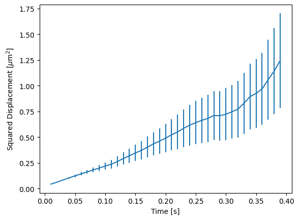
Note how the curves diverge quickly for larger time lags. Larger lags have far fewer points contributing to them. MSDs follow a gamma distribution becoming more and more Gaussian with more averaging [Mic10, MB12]. This means that smaller lags generally show a symmetric almost Gaussian distribution, while large (less averaged) lags show a much bigger variance. By simulating a large number of tracks, we can visualize this:

tracks = lk.simulation.simulate_diffusive_tracks(diffusion_constant=1.0, steps=12, dt=0.01, observation_noise=0.1, num_tracks=1500)
frame_lags = tracks[0].msd()[0]
all_msds = np.asarray([track.msd()[1] for track in tracks]).T
histogram_edges = np.arange(0, np.max(all_msds), 0.02)
msd_histogram = np.array([np.histogram(msd_frame, histogram_edges, density=True)[0] for msd_frame in all_msds])
histogram_centers = (histogram_edges[:-1] + histogram_edges[1:]) / 2

fig = plt.figure(figsize=(10, 5))
ax = fig.add_subplot(121, projection="3d")
view_limit = 0.8
for lag_time, hist in zip(frame_lags, msd_histogram):
    ax.bar(
        histogram_centers[histogram_centers < view_limit],
        hist[histogram_centers < view_limit],
        zs=lag_time,
        zdir="y",
        alpha=0.8,
        width=histogram_centers[1]-histogram_centers[0]
    )

plt.xlim([0, 0.8])
ax.view_init(20, -60)
ax.set_zticks([])
ax.set_xlabel(r'MSD [$\mu m^2$]')
ax.set_ylabel('Lag time [s]')
plt.tight_layout();

Ensemble MSD

If a group of tracks experience the same environment and diffusion coefficient, then it makes sense to compute an averaged MSD estimate using ensemble_msd():

tracks = lk.simulation.simulate_diffusive_tracks(diffusion_constant=1.0, steps=40, dt=0.01, observation_noise=0.1, num_tracks=25)
ensemble_msd = tracks.ensemble_msd()

This returns a weighted average of the TAMSDs coming from all the tracks (where the weight is determined by the number of points that contribute to each estimate). If the tracks are of equal length, this weighting will not have an effect (since all the weights will be the same). You can plot the ensemble msd as follows:

plt.figure()
ensemble_msd.plot()

Important take-aways

MSD estimates should be handled with care.

1. For larger lag times, MSD values are averaged over fewer lags. This means that the uncertainty in the MSD estimate increases with lag time.

2. Poorly averaged MSDs will show a high variance and should not be assumed to be Gaussian distributed.

3. MSDs for different lags are highly correlated and one should not fit these values as though they were independent data points unless care is taken that it is valid to do so (more on this below).

In addition, there are other experimental parameters, such as motion blur and localization accuracy that have to be accounted for. In the next sections, we will discuss various methods for diffusion analysis that take these variables into account.

Ordinary Least Squares

Real measurements are affected by noise, which leads to localization error. In addition to this, depending on the method used to detect the position of the particle, there may also be motion blur. These two sources of error manifest themselves as an offset in the MSD curve given by:

\[\mathrm{offset} = 2 \sigma^2 - 4 R D \Delta t\]

Here \(\sigma\) is the static localization uncertainty, \(R\) is a motion blur constant and \(\Delta t\) represents the time step. With pure diffusive motion (a complete absence of drift) in an isotropic medium, 1-dimensional MSDs can be fitted by the following relation:

\[\rho[n] = 2 D n \Delta t + \mathrm{offset}\]

Here \(D\) is the diffusion constant in \(\mathrm{um}^2/s\), \(\Delta t\) is the time step, \(n\) is the step index and the offset is determined by the localization uncertainty.

While it may be tempting to use a large number of lags in the diffusion estimation procedure, this actually produces poor estimates of the diffusion constant [Mic10, MB12, QSE91], because, as mentioned above, the error in the MSD value increases with lag time. There exists an optimal number of lags to fit such that the estimation error is minimal. This optimal number of lags depends on the ratio between the diffusion constant and the dynamic localization accuracy:

\[\epsilon_\mathrm{localization} = \frac{\mathrm{offset}}{\mathrm{slope}} = \frac{2 \sigma^2 - 4 R D \Delta t}{2 D \Delta t} = \frac{\sigma^2}{D \Delta t} - 2 R\]

When localization is infinitely accurate, the optimal number of points is two [Mic10]. At the optimal number of lags, it doesn’t matter whether we use a weighted or unweighted least squares algorithm to fit the curve [Mic10], and therefore we opt for the latter, analogously to [MB12]. With Pylake, you can obtain an estimated diffusion constant by invoking:

>>> tracks[0].estimate_diffusion(method="ols")
DiffusionEstimate(value=7.804440367653842, std_err=2.527045387449447, num_lags=2, num_points=80, method='ols', unit='um^2 / s')

Note that Pylake gives you both an estimate for the diffusion constant, as well as its expected uncertainty and the number of lags used in the computation. The uncertainty estimate in this case is based on Equation A1b in [BvBulowH20].

Generalized Least Squares

As mentioned above, subsequent data points in an MSD curve are highly correlated. One can account for these correlations by computing the covariance matrix of the MSD values [BvBulowH20]. This covariance matrix can then be used in the estimation procedure to determine the diffusion constant. This option is implemented under the name generalized least squares (GLS).

CoVariance-based Estimator

A third more performant and unbiased method for computing the free diffusion is the covariance-based estimator (CVE) [Ves16, VBF14]. This estimator calculates the diffusion constant directly from the displacements without calculating MSDs first. Since the CVE does not rely on computing MSDs, it avoids the complications that arise from their use.

Defining the displacements as \(\Delta x_n = x_n - x_{n + 1}\), the displacement covariance matrix is tri-diagonal [VBF14, VPMF15]:

\[\begin{split}\begin{align} \langle\left(\Delta x_n\right)^2\rangle & = & 2 D \Delta t + 2 \left(\sigma^2 - 2 R D \Delta t\right) \\ \langle\Delta x_n \Delta x_{n+1}\rangle & = & -\left(\sigma^2 - 2 R D \Delta t \right) \\ \langle\Delta x_n \Delta x_m\rangle & = & 0 \mathrm{, for }\left| n-m \right| > 1. \end{align}\end{split}\]

Here \(D\) represents the diffusion constant, \(sigma\) is the localization uncertainty standard deviation and \(R\) is the motion blur constant. In the current implementation, we assume the motion blur to be negligible for confocal scans (see note below). From these relations, one can derive the covariance based estimator [VBF14, VPMF15] for diffusion:

\[\hat{D} = \frac{\overline{\left(\Delta x_n\right)^2}}{2 \Delta t} + \frac{\overline{\Delta x_n \Delta x_{n+1}}}{\Delta t}\]

and localization uncertainty:

\[\hat{\sigma^2} = R \overline{\left(\Delta x\right)^2} + (2 R - 1) \overline{\Delta x_n \Delta x_{n+1}}\]

Here the bar indicates averaging over the time series. This method can be extended to handle tracks that have gaps due to blinking by only considering the successful localizations [Ves16]. To take this into account, we replace \(\Delta t\) with \(\overline{\Delta t_m}\), where \(t_m\) indicates the timestep between the successful localizations \(m\) and \(m+1\) [Ves16].

If the localization uncertainty is known beforehand, one can derive the following estimator:

\[\hat{D} = \frac{\overline{\left(\Delta x_n\right)^2} - 2 \sigma^2}{2 (1 - 2 R) \Delta t}\]

The performance of these covariance-based estimators can be characterized by its signal to noise ratio (SNR). This SNR is defined by:

\[\mathrm{SNR} = \frac{\sqrt{D \Delta t}}{\sigma}\]

When the SNR is larger than 1, the CVE is both optimal and fast [VBF14]. For smaller values for the SNR, we recommend using OLS or GLS instead.

Motion blur

The motion blur coefficient \(R\) is a value between 0 and 1/4 given by

\[R = \frac{1}{\Delta t} \int_{0}^{\Delta t}S(t) \left(1 - S(t)\right)dt\]

with

\[S(t) = \int_{0}^{t} c(t') dt'\]

Here, the aperture function is defined as \(c(t)\), where \(c(t)\) represents the fraction of illumination happening before time t. \(c(t)\) is normalized such that \(S(0) = 0\) and \(S(\Delta t) = 1\). For a rectangular shutter or exposure window, one obtains \(R = \frac{1}{6} \frac{t_{\mathrm{exposure}}}{\mathrm{line\_time}}\). In the current implementation we assume the motion blur constant to be negligible (zero) for confocal acquisition, since the time spent scanning over the particle is low compared to the line time.

When estimating both localization uncertainty and the diffusion constant, the motion blur factor has no effect on the estimate of the diffusion constant itself, but it does affect the calculated uncertainties. In the case of a provided localization uncertainty, it does impact the estimate of the diffusion constant itself.

Comparing the estimators on single tracks

This next section will compare the performance of the various estimators. To assess the performance, we make use of simulated tracks with a known diffusion constant. This allows studying the effect of the diffusive SNR on the accuracy (inverse of bias) and precision (inverse of variance) of the different estimators. Based on our definition of the SNR, we can conclude that the diffusion constant to achieve a specific SNR is given by:

\[D = \frac{\mathrm{SNR}^2 \sigma^2}{\Delta t}\]

For our own convenience, let’s define a small function that returns simulation parameters for a particular SNR:

# Simulation settings
def snr_to_diffusion_parameters(snr, dt=0.1, observation_noise=0.1):
    return {
        "diffusion_constant": (snr * observation_noise)**2 / dt,
        "dt": dt,
        "observation_noise": observation_noise,
    }

We can now generate diffusive tracks at varying SNRs:

plt.figure(figsize=(15, 6))
snrs = np.arange(0.5, 1.75, 0.25)
for idx, snr in enumerate(snrs):
    plt.subplot(2, len(snrs), idx + 1)
    tracks = lk.simulation.simulate_diffusive_tracks(**snr_to_diffusion_parameters(snr), steps=40, num_tracks=20)
    tracks.plot()
    plt.title(f"SNR = {snr:.2f}")
    plt.ylim([-3, 3])
    plt.subplot(2, len(snrs), idx + 1 + len(snrs))
    tracks.ensemble_msd(max_lag=10).plot()
    plt.ylim([0, 0.6])

plt.tight_layout()

We want to evaluate how well the methods work. To do this, we will generate a sample of tracks (where we know the ground truth) and apply each of the methods to it. We then divide the obtained diffusion constant by the true one. We can then see how much each method deviates from the correct estimate. We use the following function to quickly perform these numerical experiments. This function takes a method for simulating tracks and a dictionary with methods to apply to them:

def test_estimation_methods(simulate_tracks, snrs, methods):
    """Function used to test the methods.

    This function uses a simulation function to simulate tracks at various SNRs
    and then estimates diffusion constants for all the tracks.

    Parameters
    ----------
    simulation_function : callable
        Simulation function. Takes an SNR and produces simulations and a true diffusion constant.
    snrs : array_like
        SNRs to simulate for
    methods : dict of callable
        Dictionary with methods to apply to the tracks. Each dictionary
        value should be a callable that takes `KymoTracks` and returns a list
        of diffusion estimates.
    """
    results = {key: [] for key in methods.keys()}
    var_estimates = {key: [] for key in methods.keys()}

    for snr in snrs:
        # Simulate our tracks for different snrs.
        tracks, true_parameter = simulate_tracks(snr)

        for method, estimates in results.items():
            # Estimate constant for each track
            diffusion_ests = methods[method](tracks)

            # Extract diffusion constants and divide by the true value
            estimates.append([est.value / true_parameter for est in diffusion_ests])
            var_estimates[method].append([est.std_err**2 / true_parameter**2 for est in diffusion_ests])

    return results, var_estimates

This function generates a list of the estimates for each SNR for each method. To perform an analysis on the accuracy of these estimators, we need to define a simulation function and a dictionary with methods to apply to the tracks. Let’s start by comparing the single track performance of the CVE, GLS and OLS method:

methods = {
    "cve": lambda tracks: tracks.estimate_diffusion("cve"),
    "gls": lambda tracks: tracks.estimate_diffusion("gls"),
    "ols": lambda tracks: tracks.estimate_diffusion("ols"),
}

def simulate_tracks(snr):
    """Function used to simulate tracks"""
    params = snr_to_diffusion_parameters(snr)  # Determine diffusion parameters
    return lk.simulation.simulate_diffusive_tracks(**params, num_tracks=500, steps=40), params["diffusion_constant"]

snrs = 10 ** np.arange(-1, 1.1, 0.25)
results, variances = test_estimation_methods(simulate_tracks, snrs, methods)

Let’s plot the two extremes in terms of SNR:

plt.figure()

ax1 = plt.subplot(2, 1, 1)
plt.hist(results["ols"][0], 30, label="ols")
plt.hist(results["cve"][0], 30, label="cve", alpha=0.7)
plt.title(f"SNR = {snrs[0]}")
plt.ylabel("Probability density")
plt.legend()

plt.subplot(2, 1, 2, sharex=ax1)
plt.hist(results["ols"][-1], 30, label="ols")
plt.hist(results["cve"][-1], 30, label="cve", alpha=0.7)
plt.title(f"SNR = {snrs[-1]}")
plt.ylabel("Probability density")
plt.xlabel("Diffusion constant [$\mu$m/s]")
plt.xlim([-20, 20])
plt.tight_layout()

If we look at these two extremes, we see that the CVE performs very poorly at very low SNRs (very imprecise, i.e. high variance). The OLS fares better in this particular case. To study this in a bit more detail, it would be nice to plot the mean and standard deviation of all the estimators as a function of SNR. The following function can be used to convert the results we have into such a plot:

def plot_accuracy(x, data, variance=None, label="", marker=""):
    # Calculate the mean and bounds
    center = np.asarray([np.nanmean(d) for d in data])
    std = np.asarray([np.nanstd(s) for s in data])
    lb, ub = center - std, center + std

    # Plot the results
    p = plt.plot(x, center, marker=marker, label=label)
    color = p[0].get_color()  # Fetch the color so that we can make the other the same

    # label="_nolegend_" prevents a new label from being issued for each plot
    if variance:
        avg_variance = np.asarray([np.mean(v) for v in variance])
        p = plt.errorbar(x, center, np.sqrt(avg_variance), marker=marker, label="_nolegend_", color=color)

    plt.plot(x, lb, color=color, marker="", label="_nolegend_")
    plt.plot(x, ub, color=color, marker="", label="_nolegend_")
    plt.fill_between(x, lb, ub, color=color, alpha=0.1)
    plt.xscale("log")
    plt.ylabel("$\hat{D}$/D [-]")
    plt.xlabel("SNR [-]")
    plt.xlim([min(x), max(x)])
    plt.axhline(1.0, color="k", linestyle="--")
    plt.legend()

Now let’s compare the different methods for a fixed number of tracks of equal length:

plt.figure()
for method, estimates in results.items():
    plot_accuracy(snrs, estimates, variances[method], label=method)

plt.ylim([-2, 3]);

In this plot, we see the performance of the different methods. The shaded area indicates the area encapsulated by the mean ± standard deviation. It is clear from this plot that for SNR > 1 all of the methods perform equally well. We also see that the uncertainty estimates (indicated with the solid vertical lines) are pretty accurate on average. For lower SNRs, the precision quickly drops for CVE, while there is some bias for OLS.

Ensemble estimates

What if the tracks are very short? We can simulate this scenario as well:

def simulate_tracks(snr):
    """Function used to simulate tracks"""
    params = snr_to_diffusion_parameters(snr)
    tracks = lk.simulation.simulate_diffusive_tracks(**params, steps=8, num_tracks=500)
    return tracks, params["diffusion_constant"]

snrs = 10**np.arange(-1, 1.1, 0.125)
results, _ = test_estimation_methods(simulate_tracks, snrs, methods=methods)
plt.figure()
for method, estimates in results.items():
    plot_accuracy(snrs, estimates, label=method)

plt.ylim([-5, 6]);

In this case, getting precise per track estimates at low SNR is unrealistic (note the vertical axis range), since all the estimators perform poorly at low SNRs when there are only few points in the track.

However, it might be possible to still get a single good estimate for an ensemble of tracks (analyzing multiple tracks at once). With ensemble analysis we assume that the diffusion for the individual tracks is the same. How to best aggregate multiple tracks to obtain such an estimate depends depends on the method of choice.

Covariance-Based Estimator

Aggregating results for the CVE is straightforward, since those can just be obtained by performing a weighted average of the per-track results. Here the weights are chosen to be the number of points contributing to each track. This way, longer tracks contribute more to the estimate than short tracks which is beneficial for both accuracy and precision. The weighted average is computed as [VBF14]:

\[\overline{\hat{D}} = \frac{\sum_{m=1}^M N_m \hat{D}_m}{\sum_{m=1}^M N_m}\]

Here \(M\) is the number of tracks, \(D_m\) corresponds to the diffusion constant of track \(m\) while \(N_m\) corresponds to the number of data points contributing to its estimate. The associated variance of the weighted mean is given by:

\[\mathrm{var}\left(\overline{\hat{D}}\right) = \frac{\sum_{m=1}^M N_m \left(\hat{D}_m - \overline{\hat{D}}\right)^2}{\left(M - 1\right) \sum_{m=1}^M N_m}\]

To check how the performance of the ensemble estimators compares to individual track estimation, the estimation procedure becomes a bit more complex. Instead of simulating a single track many times, we simulate a collection of tracks many times and perform estimation on this. Unfortunately, this means that these notebook cells also take more time to evaluate:

def simulate_tracks(snr):
    """Function used to simulate tracks"""
    params = snr_to_diffusion_parameters(snr)
    tracks = [
        lk.simulation.simulate_diffusive_tracks(**params, steps=8, num_tracks=10)
        for _ in range(100)
    ]
    return tracks, params["diffusion_constant"]

methods = {
    "cve single": lambda list_of_tracks: [t.estimate_diffusion("cve") for tracks in list_of_tracks for t in tracks],
    "cve ensemble": lambda list_of_tracks: [t.ensemble_diffusion("cve") for t in list_of_tracks],
}

snrs = 10**np.arange(-1, 1.1, 0.125)
results, variances = test_estimation_methods(simulate_tracks, snrs, methods=methods)
plt.figure()
for method, estimates in results.items():
    plot_accuracy(snrs, estimates, variance=variances[method], label=method)

plt.ylim([-5, 6]);

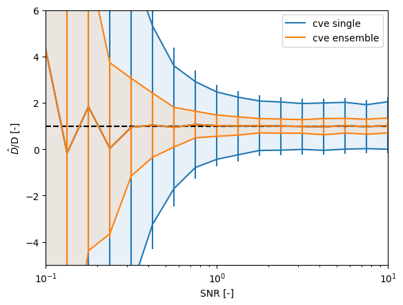
Here we simulated 10 tracks with 8 steps per track. As expected, the ensemble CVE results in a far lower variances (each estimate uses more information). The uncertainty estimate Pylake returns on the individual CVEs is a little conservative this time (vertical lines), but the ensemble uncertainty estimate is pretty accurate.

If we can safely assume that the localization uncertainty is constant then it is possible to improve the diffusion estimates by computing an ensemble averaged localization error first and then using that estimate when determining the per-track CVE. Let’s define a function that does just this and compare it to the single step CVE:

def cve_single_using_ensemble_loc_uncertainty(tracks):
    ensemble_estimate = tracks.ensemble_diffusion("cve")
    # Plug in the ensemble localization uncertainty estimates
    return tracks.estimate_diffusion(
        method="cve",
        localization_variance=ensemble_estimate.localization_variance,
        variance_of_localization_variance=ensemble_estimate.variance_of_localization_variance
    )

methods = {
    "cve single": lambda list_of_tracks: [t.estimate_diffusion("cve") for tracks in list_of_tracks for t in tracks],
    "cve single + fixed variance": lambda list_of_tracks: [t for tracks in list_of_tracks for t in cve_single_using_ensemble_loc_uncertainty(tracks)],
    "cve ensemble": lambda list_of_tracks: [t.ensemble_diffusion("cve") for t in list_of_tracks],
}

results, variances = test_estimation_methods(simulate_tracks, snrs, methods=methods)
plt.figure()
for method, estimates in results.items():
    plot_accuracy(snrs, estimates, variance=variances[method], label=method)

plt.ylim([-5, 6]);

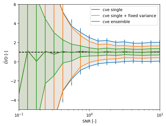
As expected, the uncertainty lies somewhere between the ensemble estimate and the individual track estimate. Note however that we would be getting this precision on a per track basis. This means that we could still use this analysis to obtain a distribution of diffusion estimates and see if there are subgroups with different diffusion constants.

MSD-based methods

For MSD based methods, simply calculating a weighted average of per-track estimates is not optimal. Estimating MSDs from very short tracks can be problematic because insufficient averaging has taken place for the individual MSDs. In such cases, the only option may be to calculate ensemble averaged MSDs and compute the diffusion constant from these.

Averaging multiple MSDs can provide a better estimate. If all included tracks have the same number of points, then averaging them doesn’t change the expected MSD. It does however reduce the variance by a factor of \(1/M\) and brings the distribution closer to a Gaussian. This follows from the fact that the MSDs follow a Gamma distribution and the additive property of independent gamma distributions [Mic10]. As a consequence, the procedure used to estimate the appropriate number of points can safely be used as long as the track lengths are roughly the same.

Working with ensemble MSDs leads to much improved estimates of the diffusion constant. We will demonstrate this, by comparing the following two procedures:

1. Averaging diffusion constants obtained by calculating them on short tracks and calculating their average (bad).

2. Performing a single estimate of a diffusion constant for a group of tracks by estimating the ensemble MSD first.

The first of these two methods is not available in Pylake directly, because it is not a recommended procedure. As such, it requires a bit more work to make sure that we save it in a similar format as Pylake does:

# Because our testing function expects a class with a value and std_err attribute
# we have to wrap our results in a similar class.
class CustomDiffusionEstimate:
    def __init__(self, value, std_err):
        self.value = value
        self.std_err = std_err

def bad_ols(tracks):
    """Just "average" the results for the tracks (NOT a good method)"""
    diffusion_estimates = tracks.estimate_diffusion("ols")
    avg_diff_est = np.mean([d.value for d in diffusion_estimates])
    std_diff_est = np.std([d.value for d in diffusion_estimates]) / np.sqrt(len(diffusion_estimates))
    return CustomDiffusionEstimate(avg_diff_est, std_diff_est)

def simulate_tracks(snr):
    """Function used to simulate tracks"""
    params = snr_to_diffusion_parameters(snr)
    tracks = [
        lk.simulation.simulate_diffusive_tracks(**params, steps=8, num_tracks=10)
        for _ in range(100)
    ]
    return tracks, params["diffusion_constant"]

methods = {
    "bad_ols": lambda list_of_tracks: [bad_ols(t) for t in list_of_tracks],
    "ols_ens": lambda list_of_tracks: [t.ensemble_diffusion("ols") for t in list_of_tracks],
}

snrs = 10**np.arange(-1, 1.1, 0.125)
results, variances = test_estimation_methods(simulate_tracks, snrs, methods=methods)
plt.figure()
for method, estimates in results.items():
    plot_accuracy(snrs, estimates, variances[method], label=method)

plt.ylim([-5, 6]);

We can see that while both result in increased precision, one is not accurate at all (highly biased) for low SNRs (the mean deviates a lot from 1).

Different track lengths

When performing real experiments, tracks are rarely the same length. In the following experiment we simulate tracks with a length coming from an exponential distribution:

def simulate_with_exponential_length(tau, params, num_tracks=10, min_length=5):
    """Simulate tracks of varying lengths

    The lengths are drawn from an exponential distribution."""
    # Redraw tracks until we get 20 above the minimum length
    lengths = np.zeros(shape=num_tracks, dtype=int)
    elements_below = lengths < min_length
    while np.any(elements_below):
        elements_below = lengths < min_length
        lengths[elements_below] = np.round(np.random.exponential(tau, size=np.sum(elements_below)) / params["dt"]).astype(int)

        group = lk.simulation.simulate_diffusive_tracks(**params, steps=max(5, lengths[0]), num_tracks=1)
        for num_points in lengths[1:]:
            group += lk.simulation.simulate_diffusive_tracks(**params, steps=max(5, num_points), num_tracks=1)

    return group

def simulate_tracks(snr):
    """Function used to simulate tracks"""
    params = snr_to_diffusion_parameters(snr)
    tracks = [
        simulate_with_exponential_length(1.1, params, num_tracks=20)
        for _ in range(100)
    ]
    return tracks, params["diffusion_constant"]

def simple_average_est(tracks, method):
    """Just "average" the results for the tracks (NOT a good method)"""
    diffusion_estimates = tracks.estimate_diffusion(method)
    avg_diff_est = np.mean([d.value for d in diffusion_estimates])
    std_diff_est = np.std([d.value for d in diffusion_estimates]) / np.sqrt(len(diffusion_estimates))
    return CustomDiffusionEstimate(avg_diff_est, std_diff_est)

methods = {
    "cve single": lambda list_of_tracks: [t.estimate_diffusion("cve") for tracks in list_of_tracks for t in tracks],
    "gls single": lambda list_of_tracks: [t.estimate_diffusion("gls") for tracks in list_of_tracks for t in tracks],
    "ols single": lambda list_of_tracks: [t.estimate_diffusion("ols") for tracks in list_of_tracks for t in tracks],
    "cve unweighted": lambda list_of_tracks: [simple_average_est(t, "cve") for t in list_of_tracks],
    "cve ensemble": lambda list_of_tracks: [t.ensemble_diffusion("cve") for t in list_of_tracks],
    "ols ensemble": lambda list_of_tracks: [t.ensemble_diffusion("ols") for t in list_of_tracks],
}

snrs = 10**np.arange(-1, 1.1, 0.125)
results, variances = test_estimation_methods(simulate_tracks, snrs, methods=methods)

plt.figure(figsize=(12, 4))
plt.subplot(1, 2, 1)
for method in ("ols single", "gls single", "cve single"):
    plot_accuracy(snrs, results[method], variance=variances[method], label=method)
plt.title("Single track estimates")
plt.ylim([-1, 3])

plt.subplot(1, 2, 2)
for method in ("cve unweighted", "cve ensemble", "ols ensemble"):
    plot_accuracy(snrs, results[method], variance=variances[method], label=method)
plt.title("Ensemble estimates")
plt.ylim([-1, 3]);

We can see that the ensemble estimates fare quite well in this case, while the single estimates show a large variability. A lot of this variability in the individual estimates comes from short tracks. We can show this by including a filtering step (requiring a minimum track length). We can filter tracks shorter than a certain length by using filter_tracks():

min_length = 10
methods = {
    "cve single": lambda list_of_tracks: [t.estimate_diffusion("cve") for tracks in list_of_tracks for t in tracks],
    "ols single": lambda list_of_tracks: [t.estimate_diffusion("ols") for tracks in list_of_tracks for t in tracks],
    "cve (filtered)": lambda list_of_tracks: [t.estimate_diffusion("cve") for tracks in list_of_tracks for t in lk.filter_tracks(tracks, minimum_length=min_length)],
    "ols (filtered)": lambda list_of_tracks: [t.estimate_diffusion("ols") for tracks in list_of_tracks for t in lk.filter_tracks(tracks, minimum_length=min_length)],
    "cve ensemble": lambda list_of_tracks: [t.ensemble_diffusion("cve") for t in list_of_tracks],
    "ols ensemble": lambda list_of_tracks: [t.ensemble_diffusion("ols") for t in list_of_tracks],
    "cve ensemble (filtered)": lambda list_of_tracks: [lk.filter_tracks(t, minimum_length=min_length).ensemble_diffusion("cve") for t in list_of_tracks],
    "ols ensemble (filtered)": lambda list_of_tracks: [lk.filter_tracks(t, minimum_length=min_length).ensemble_diffusion("ols") for t in list_of_tracks],
}

snrs = 10**np.arange(-1, 1.1, 0.125)
results, variances = test_estimation_methods(simulate_tracks, snrs, methods=methods)

plt.figure(figsize=(12, 4))
plt.subplot(1, 2, 1)
for method in ("cve single", "ols single", "cve (filtered)", "ols (filtered)"):
    plot_accuracy(snrs, results[method], variance=variances[method], label=method)
plt.ylim([-1, 3])

plt.subplot(1, 2, 2)
for method in ("cve ensemble", "ols ensemble", "cve ensemble (filtered)", "ols ensemble (filtered)"):
    plot_accuracy(snrs, results[method], variance=variances[method], label=method)
plt.ylim([-1, 3]);

The good news is that the ensemble estimates are pretty robust to filtering short tracks. This is expected since these estimates already incorporate weighting (assigning lower weight to short tracks). The bad news is that the variance for low SNR is still very high, while the method with the most precision at low SNR (OLS) is very biased. Unfortunately, what this means is that we either need to settle for ensemble estimates, or accept high variance results.

Concluding remarks

When the SNR and the number of points per track is high, all methods presented here perform well. In this case, the recommendation is to use CVE, while carrying over the localization uncertainty from the ensemble estimate. Choosing this option will allow the study of diffusion constants for individual tracks with the largest precision.

When the SNR is low, but per track estimates are required, restrict to long tracks if possible (refine the tracks and filter short tracks out) and use OLS.

If the uncertainty in the diffusion estimates is still too large, but the expectation is that the diffusion constants for different tracks are the same, consider using ensemble averages and compare ensemble averages obtained with CVE and OLS. Ensemble estimates perform well down to relatively low SNR. Note that an extra requirement for OLS is that the diffusive tracks are roughly equally long.