Introduction
This chapter gives an introduction to diffusion and an overview of the recommended methods for diffusion analysis available in Pylake. Rather than on math or syntax, this page focusses on the underlying ideas, providing an introduction for anyone who wants to start analyzing a kymograph with a diffusive protein.
Target search
Proteins diffusing through a cell often have to search for a target on DNA. A long-standing question in biology is how proteins find their target on the huge genome through random, diffusive motion. The first hypothesis was that proteins diffuse through the cytoplasm (in 3D), until they find their target. Berg and von Hippel were the first to demonstrate that the Lac repressor finds its target faster than can be explained by 3D diffusion alone. Now, many experiments have shown that proteins often alternate between diffusion in 3D (in the cytoplasm) and in 1D (along DNA). The combination of 1D and 3D diffusion is referred to as ‘facilitated diffusion’ [BB76, BWVH81] and is more efficient than 3D diffusion alone.
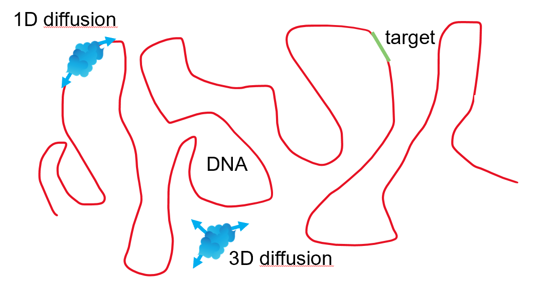
1D diffusion can directly be visualized by holding a force-stretched DNA between optically trapped beads and observing a fluorescently labelled protein bind and move along this DNA. Pylake has many functions implemented for analyzing data from such an assay. This chapter focusses on the analysis of kymographs with a protein diffusing along DNA, as in the figure below.

The diffusion coefficient
A purely diffusive protein on DNA has the same probability to move to the right as to the left, therefore the average displacement is zero. Over time, the protein will explore larger and larger regions of DNA. The diffusion coefficient (D) quantifies how fast a protein explores its environment. For example, the orange track in the figure below has a higher diffusion coefficient than the blue track. The diffusion coefficient has units of \(length^{2}/s\). For 1D diffusion along DNA, D is often expressed in \(µm^{2}/s\) or \(kbp^{2}/s\) [KHL+09].

Methods for obtaining the diffusion coefficient
The first step for analyzing a diffusive protein from a kymograph, is to track each binding event, which is further discussed below. The resulting tracks give the positions of each bound protein over time. These tracks can then be analyzed further to determine the diffusion coefficient. Below we discuss two methods for diffusion analysis that are available in Pylake.
Mean Squared Displacement analysis
A common method for determining the diffusion coefficient, is to first compute the mean squared displacement (MSD) as a function of lag time for each track. For purely diffusive motion, the first part of the MSD curve is linear, with the slope proportional to the diffusion coefficient. For 1D diffusion the MSD is given by: \(MSD = 2D\Delta t\). The diffusion coefficient can be obtained by fitting a linear function to the MSD curve, as illustrated in the figure below (simulated data):

Note that for the MSD curve, the ‘lag time’ (aka ‘time interval’) is given on the x-axis, rather than ‘time’. To compute the MSD for a certain lag time, you scan over a track, one data point at a time and compute the displacement squared from that time until that time + the lag time. So each point on the MSD curve, is an average of displacements squared for a specific lag time, see this section for the equation for the MSD.
The largest possible lag time is the duration of a track and the shortest possible lag is the time resolution, the line time of the kymograph. The image above does not show the complete MSD curve; the longest possible lag time would be 2500 seconds, but the MSD curve is only given up to a lag time of 5 seconds. The full MSD curve looks as follows:

As you can see, the full MSD curve becomes less and less linear for larger lag times. The non-linear shape of the MSD curve for large lag times is caused by:
The MSD at shorter time lags is averaged over more lags and therefore more accurate
Consecutive data points in the MSD are highly correlated
The MSD curve for larger lags is clearly not suitable for a linear fit. An important step in MSD analysis, is therefore to determine which number of lags is optimal for a linear fit and obtaining the diffusion coefficient. Taking too many lags, may result in an MSD curve that is not fully linear, while taking too little lags may not give enough data points for a good estimate of the diffusion coefficient. There are various methods for determining the optimal number of lags. The method recommended in Pylake automatically determines the optimal number of lags for you [MB12] (named ‘OLS’ in Pylake).
Covariance Based Estimator
The Covariance Based Estimator (‘CVE’) in Pylake is a method for determining the diffusion coefficient that does not rely on the MSD [TGEJ+22, Ves16, VBF14]. This method directly computes the diffusion coefficient from the displacements; there is no fitting involved. For the full equation, see this section.
Comparing CVE and MSD analysis
When tracks are long and diffusion clearly dominates over noise, CVE and MSD analysis perform equally well. The advantage of MSD analysis, is that it can be used to quantify anomalous diffusion (further discussed below). A disadvantage of MSD analysis is that it can have a small bias when applied to very short tracks, or when the diffusion coefficient is very small (when a method is biased, the diffusion coefficient obtained via that method deviates from the real diffusion constant). CVE on the other hand, is an unbiased method for determining the diffusion coefficient, but is only used for analysis of free (non-anomalous) diffusion. For a more detailed comparison between the performance of CVE and MSD analysis, see here.
Ensemble Based Estimate
The estimate of the diffusion coefficient can further be improved by using an ensemble estimate. For an ensemble estimate using MSD, Pylake averages the MSD for each lag time and combines them into one MSD curve. This MSD can then be fitted to obtain the diffusion coefficient. For CVE, Pylake computes the average diffusion coefficient of all tracks, where each track is weighted by the number of data points. An example of how to compute the ensemble estimate using CVE is given here and a comparison between using single and ensemble estimates can be found here.
Tracking a diffusive protein
Pylake has built-in tracking algorithms to track binding events on a kymograph over time. For more details on how to use the tracking algorithm in Pylake, see the Kymotracking tutorial and specifically the section on diffusion regarding diffusion analysis on kymographs. After tracking, it is possible to further improve the estimate of the positions and time coordinates of the tracks through refinement.
Refinement
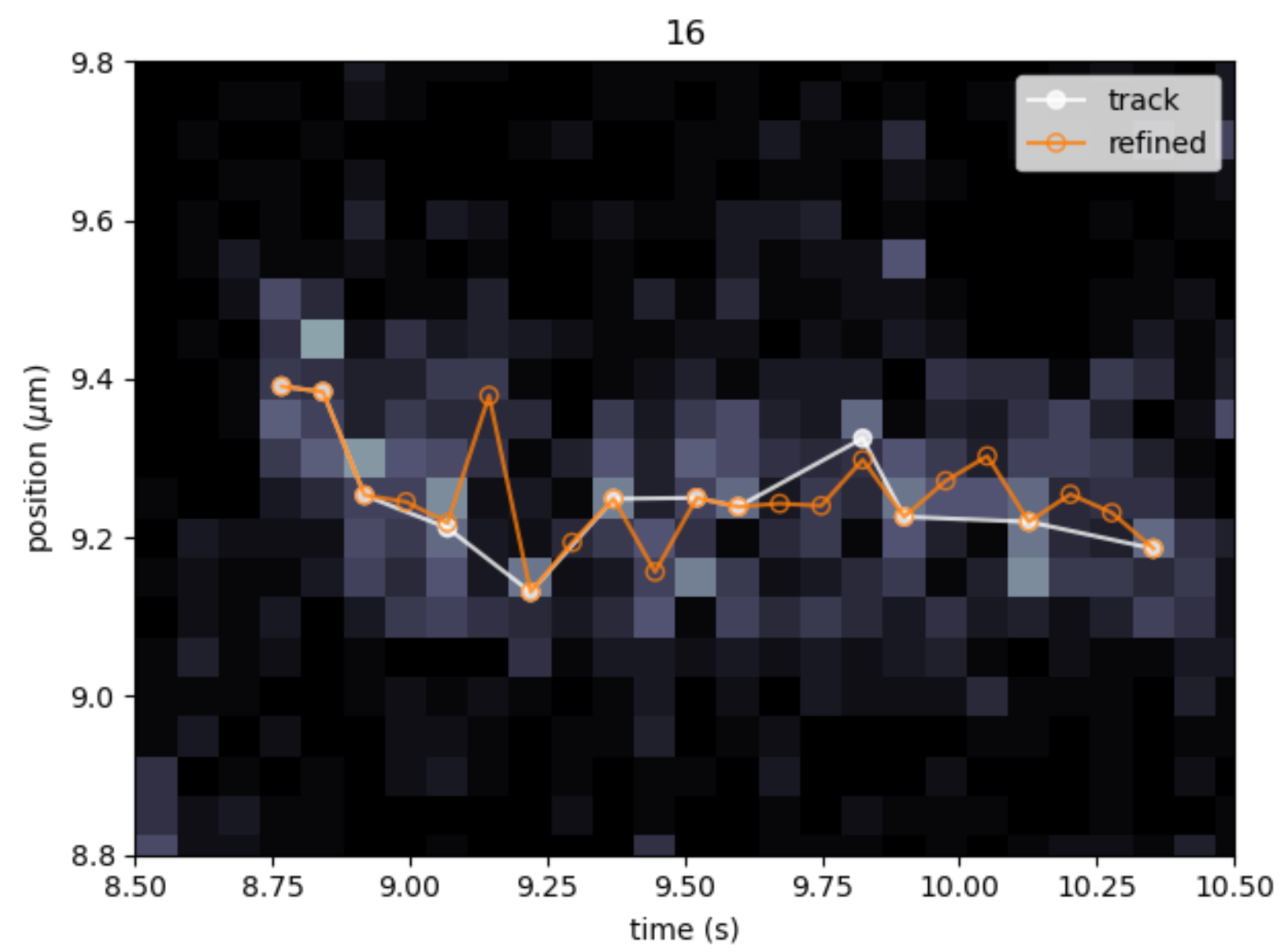
The tracking algorithm in the Pylake kymotracker does not always move from one pixel to the next, but sometimes skips a few pixels within a track. In the figure below for example, the track (white) sometimes skips one or multiple pixels. The missing frames can be added through refinement. Further, refinement can slightly improve the position estimate of a track. (The default tracking algorithm already has subpixel accuracy). The orange line shows the update of the coordinates after refining the white track.
Note that refining missing frames is recommended for MSD analysis, but not necessary for CVE. MSD analysis works best when the time between all data points is the same.
Pylake has two methods on refinement:
Centroid refinement
The method ‘Centroid refinement’ can be used to refine missing frames after tracking. The disadvantage of this method, is that it does not perform well when tracks are close together or with high background. At the moment, this method is the default in the kymotracker, because it is fast.
Gaussian refinement
Gaussian refinement fits a Gaussian function to improve the position estimate of a track and can also
refine missing frames. The advantage of this method is that it is better at refining tracks that are
close together or have a high background. Refining missing frames is not the default. When doing MSD
analysis, you have to activate the refinement of missing frames, by setting refine_missing_frames = True
(see section on gaussian refinement). After refinement, it is
good practise to inspect the refined peaks. This can be done using
KymoTrack.plot_fit() or
KymoTrackGroup.plot_fit() and
is illustrated here.
Miscellaneous
Negative diffusion coefficients
Depending on the method used for diffusion analysis, a diffusion coefficient of a single track may sometimes be negative. For example, when a diffusion coefficient is low, some diffusion coefficients are above and some below zero. The negative values do not have a biological meaning by themselves, but the average of all the diffusion coefficients from different tracks should still give a good, positive-valued estimate of the diffusion coefficient (provided that you have enough tracks, and that the protein is diffusing freely). The negative data points should not be removed from the dataset, otherwise you get a bias in the estimate of the diffusion coefficient [MB12].
Confined diffusion
If many diffusive proteins bind to the DNA at once and they are not able to pass each other, the proteins will confine each others motion, resulting in sub-diffusive or confined diffusive behavior. If you are interested in free diffusion of a protein, it is therefore best to keep the density of protein binding events low enough, such that the proteins don’t meet often. When the DNA is held between two beads in an optical tweezer experiment, the beads can also confine the motion of a diffusive protein if the protein diffuses close to the beads. If you want to exclude the effect of the beads, you can consider cutting the tracks to exclude the part where the protein reaches the bead. Another approach is to account for the presence of the beads when analyzing the data, but this option is not available in Pylake at the moment.
Fluctuating DNA
Though the DNA in an optical tweezer experiment is constrained, it still fluctuates. The motion of the DNA sets a lower limit on what diffusion coefficient can be observed for a protein diffusing along the DNA. A typical approach is to measure the diffusion coefficient of a static protein or marker and use this as a reference for the minimal observable diffusion coefficient (see for example [KDN22]).
Anomalous Diffusion
If a protein is hindered, for example by obstacles, it can not diffuse freely anymore, and the MSD curve will look different. A protein that has some motor activity will also have a differently shaped MSD curve. In both cases, we would refer to the motion as ‘anomalous diffusion’. At the moment, Pylake does not have functionality for analyzing anomalous diffusion. Usually, anomalous diffusion is analyzed by looking at the shape of the MSD curve.