12. Piezo Tracking
Download this page as a Jupyter notebook
In this tutorial, we will determine the high frequency distance (piezo distance) between the beads from the piezo mirror position of trap 1 and the corresponding force data. We will also show how to use the same reference curve to apply baseline correction for force signals in post processing.
We can download the data needed for this tutorial directly from Zenodo using Pylake.
Since we don’t want it in our working folder, we’ll put it in a folder called "test_data":
filenames = lk.download_from_doi("10.5281/zenodo.7729775", "test_data")
12.1. Trap Positional Calibration
The first step is to calibrate the high frequency trap position from the piezo mirror to the low frequency bead-to-bead distance measured by the camera.
For this calibration, we require a dataset (acquired in the absence of a tether) in which trap 1 is moved over the entire distance range intended for the experiment. The exported data file must contain the trap 1 position and camera-based distance channels.
Note
Note that this dataset should be acquired such that the bead tracking templates do not overlap. In case of overlap, make sure to first slice the position and distance data such that this region is not included.
Let’s load this dataset and perform the distance calibration by invoking:
no_tether_data = lk.File("test_data/piezo_tracking_no_tether.h5")

distance_calibration = lk.DistanceCalibration(
    no_tether_data["Trap position"]["1X"], no_tether_data.distance1, degree=2
)
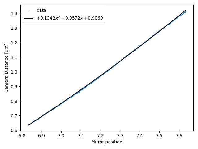
This class performs a polynomial regression between the trap position and bead tracking distance.
Note that this bead-to-bead distance already has the bead radius subtracted, therefore it reflects the surface-to-surface distance.
We can plot what this curve looks like by invoking plot() on it:
plt.figure()
distance_calibration.plot()
plt.show()
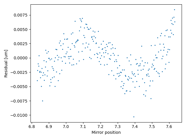
We can also inspect the residual, to determine how well the calibration model describes the data. We can see that there is some error (the discrepancy does not scatter randomly around zero), but for this experiment, 15 nm error is within an acceptable range:
plt.figure()
distance_calibration.plot_residual()
plt.show()
12.2. Baseline correction
Let’s have a look at the force data:
plt.figure()
plt.subplot(2, 1, 1)
no_tether_data.force1x.plot()
no_tether_data.force2x.plot()

plt.subplot(2, 1, 2)
no_tether_data.distance1.plot()
plt.tight_layout()
plt.show()
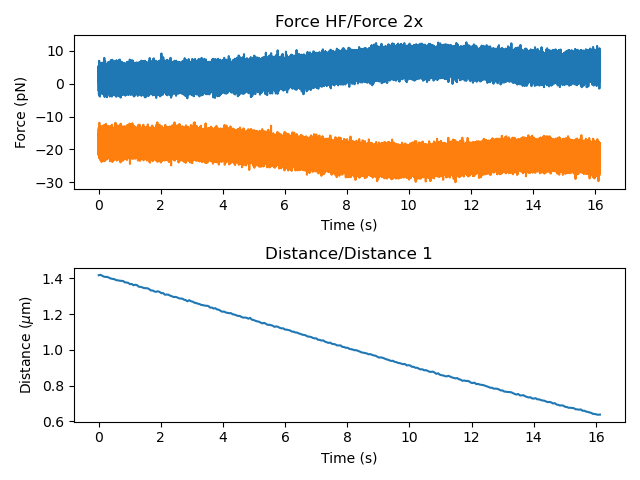
It seems that the force was not zeroed at the start of this experiment, but we can correct this in post-processing. We want to use the force when the beads are far apart (no interaction between them) which corresponds the beginning of the data. In this case, we’ll use a quarter of a second:
f1_offset = np.mean(no_tether_data.force1x[:"0.25s"].data)
f2_offset = np.mean(no_tether_data.force2x[:"0.25s"].data)
Let’s correct our force data before we use it:
background_force1x = no_tether_data.force1x - f1_offset
background_force2x = no_tether_data.force2x - f2_offset
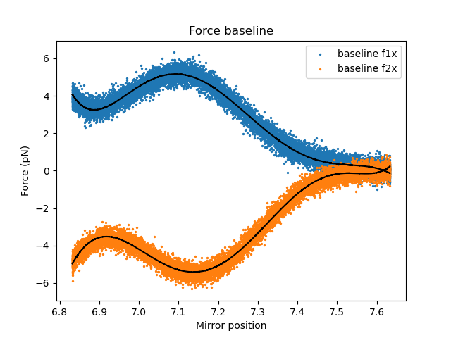
Even without a tether, the measured force can be non-zero when the beads are close together due to trap/trap interactions. We can characterize this baseline force so that it can be subtracted from our experiment force data. In principle, this step is optional, but it can greatly improve the accuracy of your force-distance curves. We can quickly determine a polynomial baseline for both traps by invoking:
baseline_1x = lk.ForceBaseLine.polynomial_baseline(
    no_tether_data['Trap position']['1X'], background_force1x, degree=7, downsampling_factor=100
)
baseline_2x = lk.ForceBaseLine.polynomial_baseline(
    no_tether_data['Trap position']['1X'], background_force2x, degree=7, downsampling_factor=100
)
Similarly as before, we can plot the fits to verify that they describe the data well:
plt.figure()
baseline_1x.plot(label="baseline f1x")
baseline_2x.plot(label="baseline f2x")
plt.legend()
plt.show()
And the residuals:
plt.figure()
baseline_1x.plot_residual(label="baseline f1x")
baseline_2x.plot_residual(label="baseline f2x")
plt.legend(loc='lower right')
plt.show()
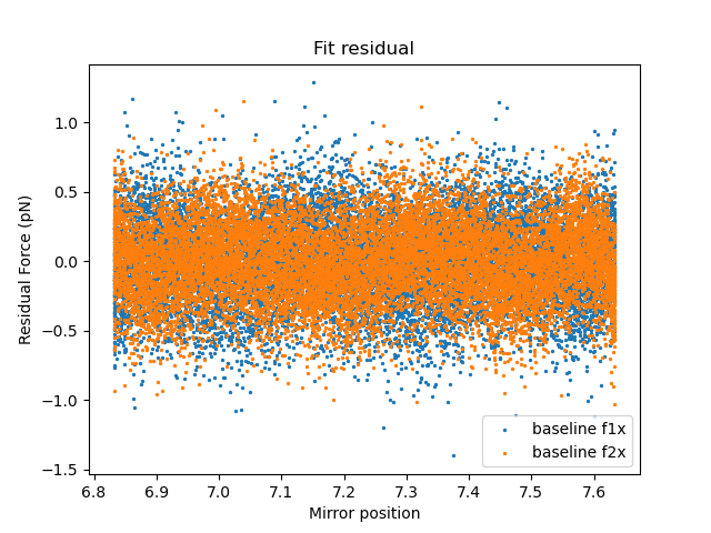
The residuals should ideally look like noise distributed around zero.
12.3. Calculating the force-dependent bead displacements
When a tether is present, it exerts a force on the beads resulting in a displacement of the beads from the trap centers. If there are only small excursions from the trap center, this displacement is assumed linear with respect to force (proportional to the trap stiffness \(\kappa\)). Therefore, we can compute the bead displacement \(\delta x\) directly from the force signal.
Thus the surface-to-surface distance between the beads can be computed by correcting the trap-based distance with the correlated force data and their respective trap stiffnesses as follows.
Here \(d_\mathrm{piezo}\) is the piezo distance and \(d_\mathrm{no\_tether}\) is the calibrated surface-to-surface distance without the tether. \(F_{1x}\) and \(F_{2x}\) are the forces measured on the beads and \(\kappa_{1x}\) and \(\kappa_{2x}\) are the trap stiffness for each trap.
To do this in Pylake, we set up the piezo distance calibration as follows:
piezo_calibration = lk.PiezoForceDistance(distance_calibration, baseline_1x, baseline_2x, signs=(1, -1))
where signs specifies the sign of force 1x and force 2x respectively. You can determine the signs by viewing the respective force channels; the channel that becomes more negative as force increases requires a -1 sign.
We now have all the calibrations we need to do piezo tracking on our experimental data.
12.4. Calculating the Fd Curve
First, we load the data acquired in the presence of a tether:
pulling_curve = lk.File("test_data/piezo_tracking_tether.h5")
And determine the piezo distance and corrected force:
tether_length, corrected_force_1x, corrected_force_2x = piezo_calibration.force_distance(
    pulling_curve['Trap position']['1X'], pulling_curve.force1x - f1_offset, pulling_curve.force2x - f2_offset, downsampling_factor=100
)
force_data = - corrected_force_2x
Here the downsampling factor determines how much the data is downsampled prior to piezo-tracking and baseline correction.
Which we can then plot:
plt.figure()
plt.scatter(tether_length.data, force_data.data, s=1)
plt.xlabel(r'Distance [$\mu$m]')
plt.ylabel('Force [pN]')
plt.show()
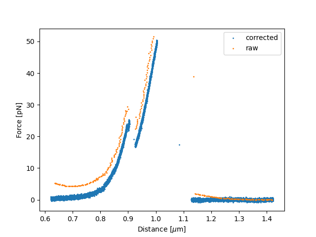
We can compare this to the camera-based distance and raw force curve and see a clear difference:
plt.figure()
plt.scatter(tether_length.data, force_data.data, s=1, label="corrected")
plt.scatter(pulling_curve.distance1.data, - (pulling_curve.downsampled_force2x.data - f2_offset), s=1, label="raw")
plt.xlabel(r'Distance [$\mu$m]')
plt.ylabel('Force [pN]')
plt.legend()
plt.show()