10.6. Low level API

Download this page as a Jupyter notebook

For those who want an API that is a little more composable, Pylake also offers a low level API to perform force calibration. This API is intended for advanced users and separates the steps of creating a power spectrum and fitting models to it.

10.6.1. Obtaining the power spectrum

First we need the data in volts as shown in previous tutorials:

filenames = lk.download_from_doi("10.5281/zenodo.7729823", "test_data")
f = lk.File("test_data/passive_calibration.h5")

force_slice = f.force1x[f.force1x.calibration[1]]
old_calibration = force_slice.calibration[0]

volts = force_slice / old_calibration.force_sensitivity

To use the more manual lower-level API, we first need the power spectrum to fit. To compute a power spectrum from our data we can invoke calculate_power_spectrum():

power_spectrum = lk.calculate_power_spectrum(volts.data, sample_rate=volts.sample_rate)

This function returns a PowerSpectrum which we can plot:

plt.figure()
power_spectrum.plot()
plt.show()

The power spectrum is smoothed by downsampling adjacent power spectral values, a procedure known as blocking. Downsampling the spectrum is required to fulfill some of the assumptions in the fitting procedure, but it comes at the cost of spectral resolution. One must be careful that the shape of the power spectrum is still sufficiently preserved. If the corner frequency is very low then downsampling too much can lead to biases in the calibration parameters. In such cases, it is better to either measure a longer interval to increase the spectral resolution or reduce num_points_per_block, the number of points used for blocking.

The range over which to compute the spectrum can be controlled using the fit_range argument. One can also exclude specific frequency ranges from the spectrum with excluded_ranges which can be useful if there are noise peaks in the spectrum. Let’s see which ranges were excluded in our Bluelake calibration:

old_calibration

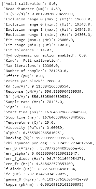
Here, they are listed in the excluded_ranges field. To reproduce the result obtained with Bluelake, these should be excluded from the power spectrum:

power_spectrum = lk.calculate_power_spectrum(
    volts.data,
    sample_rate=volts.sample_rate,
    fit_range=(1e2, 23e3),
    num_points_per_block=2000,
    excluded_ranges=old_calibration.excluded_ranges
)

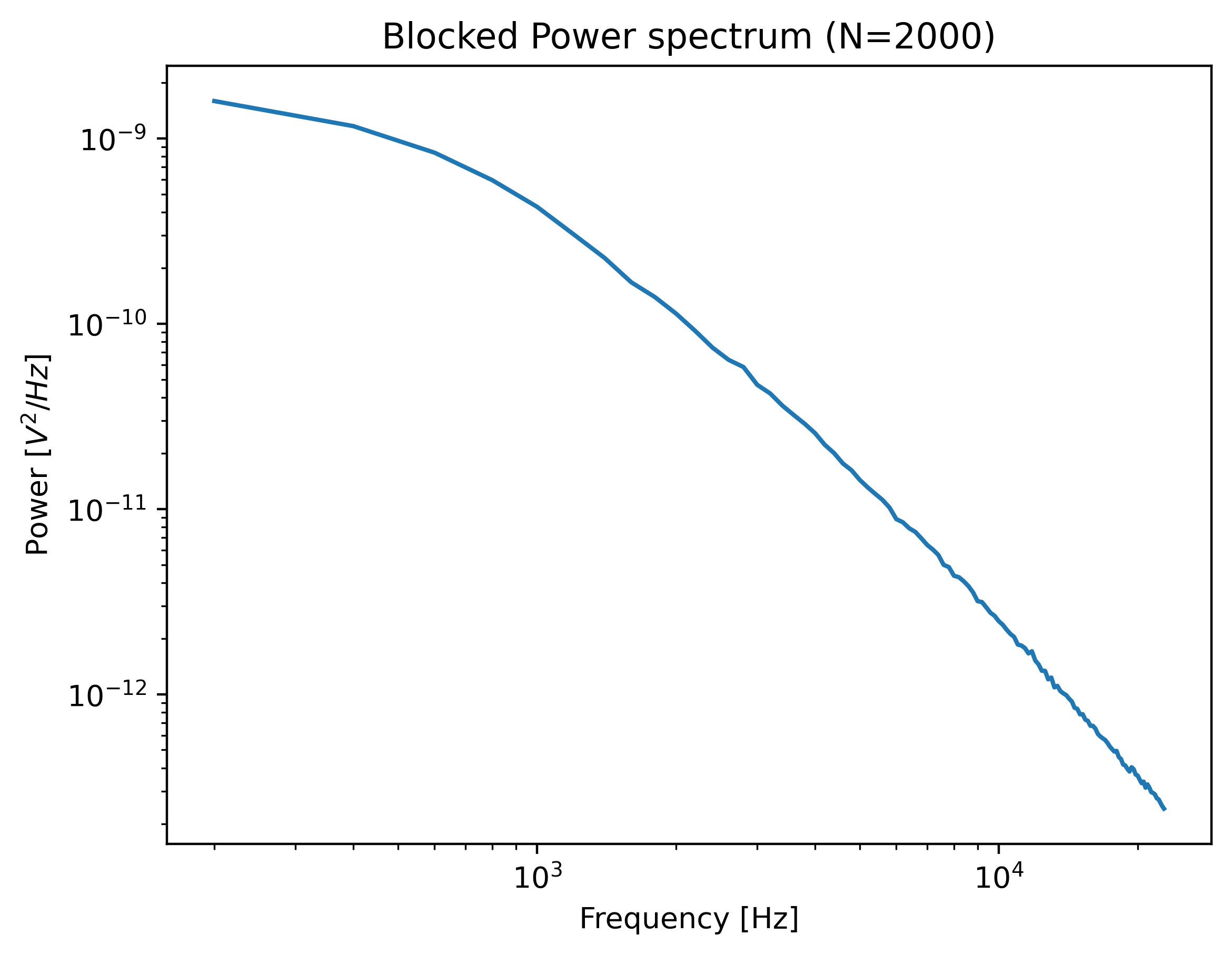
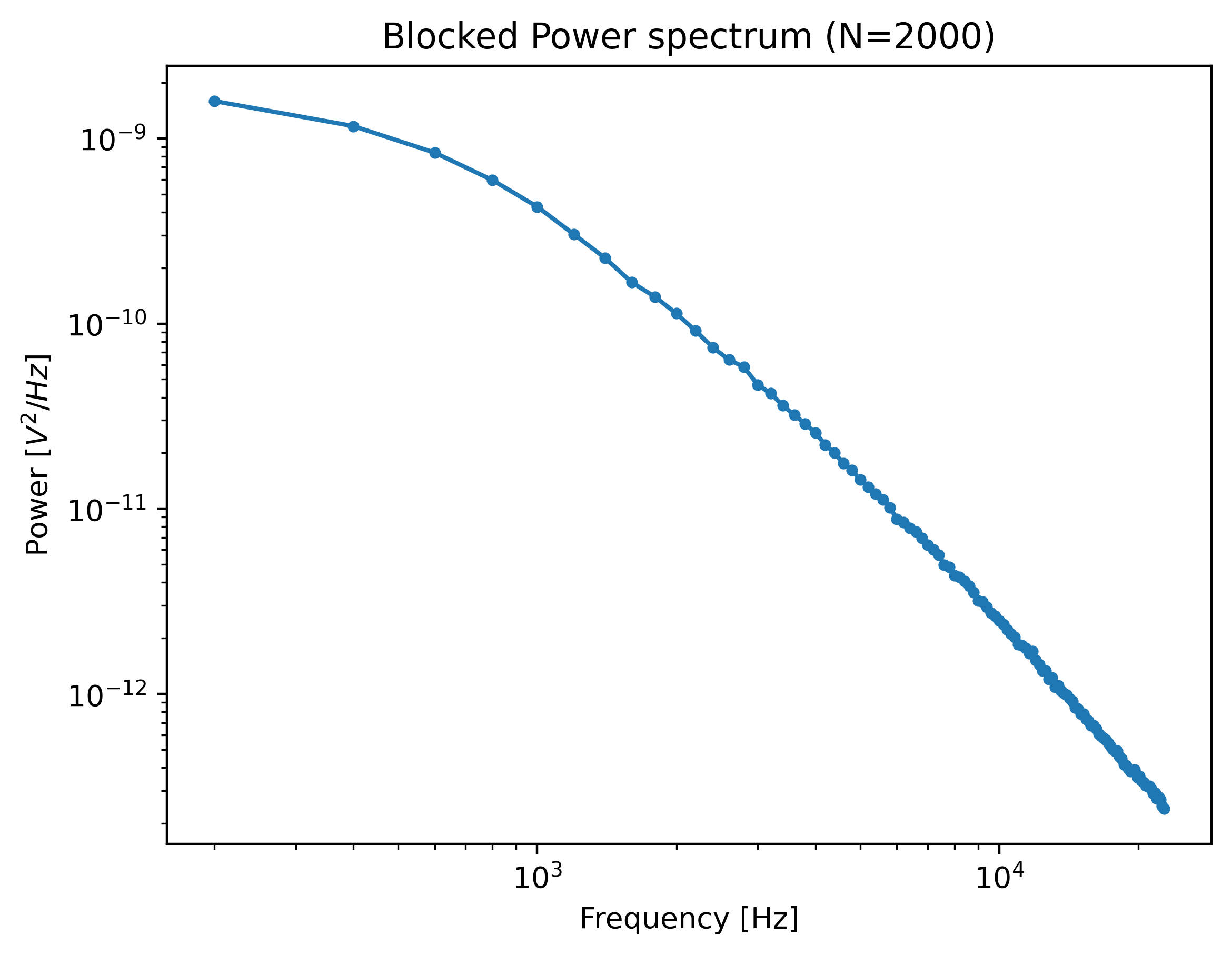
plt.figure()
power_spectrum.plot(marker=".")
plt.show()

Note that exclusion ranges are excluded prior to downsampling. Considering that a noise peak may be very narrow, it is beneficial to lower the number of points per block temporarily to find the exact exclusion range. After determination of this exclusion range, the number of points per block can be increased again. However, also see robust fitting for an automated peak identification routine.

10.6.2. Passive calibration

In the low level API, we create the model to fit the data explicitly. The next step is setting up the calibration model:

bead_diameter = old_calibration["Bead diameter (um)"]
force_model = lk.PassiveCalibrationModel(bead_diameter, temperature=25)

To fit this model to the data use fit_power_spectrum():

calibration = lk.fit_power_spectrum(power_spectrum, force_model)
calibration

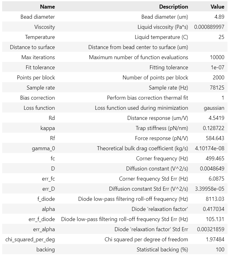
This will produce a table with your fitted calibration parameters. These parameters can be accessed as follows:

>>> print(calibration["kappa"].value)
>>> print(f.force1x.calibration[1]["kappa (pN/nm)"])
0.12872206853860946
0.1287225353482303

Note

Note that by default, a bias correction is applied to the fitted results [NF10]. This bias correction is applied to the diffusion constant and amounts to a correction of \(\frac{N}{N+1}\), where \(N\) refers to the number of points used for a particular spectral data point. It can optionally be disabled by passing bias_correction=False to fit_power_spectrum().

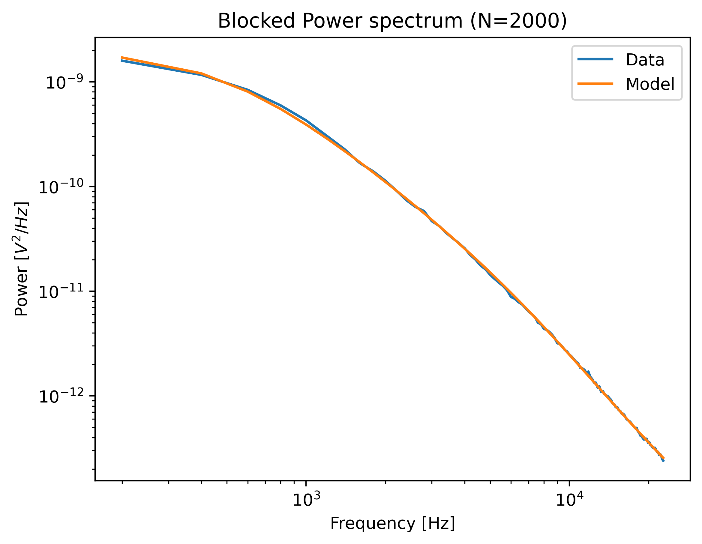
We can plot the calibration by calling:

plt.figure()
calibration.plot()
plt.show()

We can set up a model for passive calibration using the hydrodynamically correct theory according to:

force_model = lk.PassiveCalibrationModel(
    bead_diameter,
    hydrodynamically_correct=True,
    rho_sample=999,
    rho_bead=1060.0
)

Note that when rho_sample and rho_bead are omitted, values for water and polystyrene are used for the sample and bead density respectively.

10.6.2.1. Active calibration

Let’s load some active calibration data:

lk.download_from_doi("10.5281/zenodo.7729823", "test_data")
f = lk.File("test_data/near_surface_active_calibration.h5")

volts = f.force1x / f.force1x.calibration[0].force_sensitivity
bead_diameter = f.force1x.calibration[0].bead_diameter
distance_to_surface = 1.04 * bead_diameter
driving_data = f["Nanostage position"]["X"]

Instead of using the PassiveCalibrationModel presented in the previous section, we now use the ActiveCalibrationModel. We also need to provide the sample rate at which the data was acquired, and a rough guess for the driving frequency. Pylake will find an accurate estimate of the driving frequency based on this initial estimate (provided that it is close enough):

active_model = lk.ActiveCalibrationModel(
    driving_data.data,
    volts.data,
    driving_data.sample_rate,
    bead_diameter,
    driving_frequency_guess=38,
    distance_to_surface=distance_to_surface,
    driving_sample_rate=driving_data.sample_rate,
)

The rest of the procedure is the same:

power_spectrum = lk.calculate_power_spectrum(
    volts.data,
    sample_rate=volts.sample_rate,
    fit_range=(1e2, 23e3),
    num_points_per_block=2000,
)

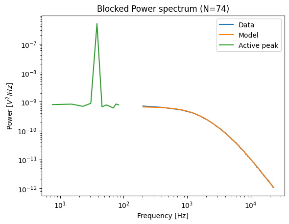
calibration = lk.fit_power_spectrum(power_spectrum, active_model)
calibration.plot(show_active_peak=True)