10.7. Robust fitting

Download this page as a Jupyter notebook

So far, we have been using least-squares fitting routines for force calibration. In that case, we assume that the error in the power at each frequency is distributed according to a Gaussian distribution. Blocking or windowing the power spectrum ensures that this assumption is close enough to the truth such that the fit provides accurate estimates of the unknown parameters. Occasionally, the power spectrum might show a spurious noise peak. Such a peak is an outlier in the expected behavior of the spectrum and therefore interferes with the assumption of having a Gaussian error distribution. As a result, the fit is skewed. In those cases, it can be beneficial to do a robust fit.

When a robust fit is performed, one assumes that the probability of encountering one or multiple outliers is non-negligible. By taking this into account during fitting, the fit can be made more robust to outliers in the data.

One downside of this approach is that the current implementation does not readily provide standard errors on the parameter estimates and that it leads to a small bias in the fit results for which Pylake has no correction.

Robust fitting can be used in combination with a least-squares fit to identify outliers automatically in order to exclude these from a second regular least-squares fit. The following example illustrates the method.

To see this effect, let’s load a dataset of uncalibrated force sensor data of a 4.4 μm bead showing Brownian motion while being trapped. In particular, look at the Force 2y sensor signal:

filenames = lk.download_from_doi("10.5281/zenodo.7729823", "test_data")
f = lk.File("test_data/robust_fit_data.h5")
f2y = f.force2y

First create a power spectrum without blocking or windowing for later use. Then derive a power spectrum with blocking from the first power spectrum:

ps = lk.calculate_power_spectrum(f2y.data, sample_rate=f2y.sample_rate, num_points_per_block=1, fit_range=(10, 23e3))
ps_blocked = ps.downsampled_by(200)

First use a passive calibration model using the hydrodynamically correct model to perform a least-squares fit and plot the result:

model = lk.PassiveCalibrationModel(4.4, temperature=25.0, hydrodynamically_correct=True)
fit = lk.fit_power_spectrum(ps_blocked, model)

plt.figure()
fit.plot()
plt.title(
    f"Skewed fit: $f_c$ = {fit.results['fc'].value:.1f}, "
    f"$D$ = {fit.results['D'].value:.4f}, "
    f"$f_d$ = {fit.results['f_diode'].value:.1f}"
)
plt.show()

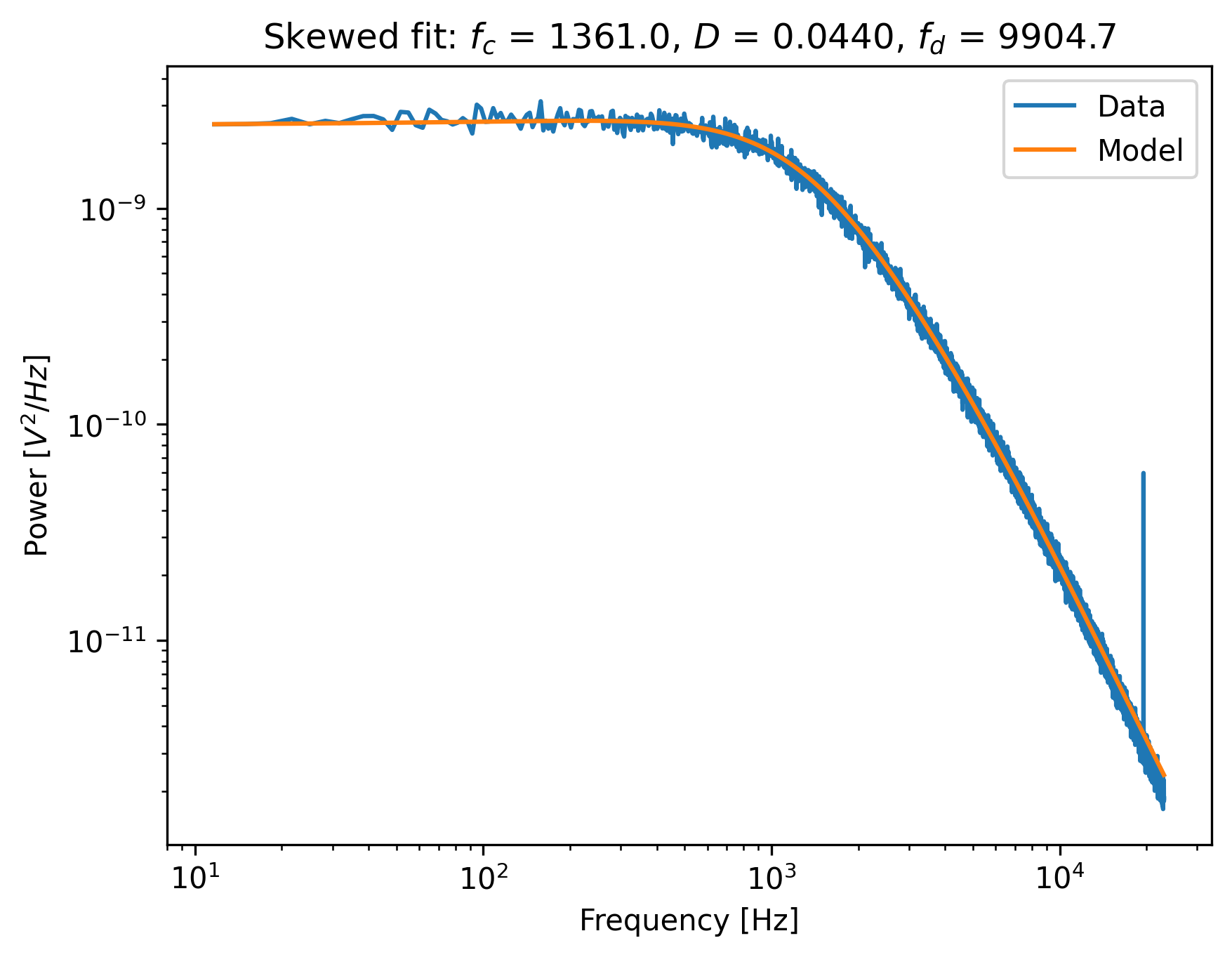
Notice how the tail of the model is skewed towards the peak, in order to reduce the least-squares error. In this case, the free parameters to fit the diode filter contribution are ‘abused’ to reduce the error between the model and the outlier. This results in biased parameter estimates.

Now do a robust fit. We do this by specifying a loss function in fit_power_spectrum(). For least-squares fitting, the loss function is 'gaussian', which is the default if nothing is specified. However, if we specify 'lorentzian', a robust fitting routine will be used instead. Because bias_correction and robust fitting are mutually exclusive, we need to explicitly turn it off:

fit = lk.fit_power_spectrum(ps_blocked, model, bias_correction=False, loss_function="lorentzian")

Now plot the robust fit:

plt.figure()
fit.plot()
plt.title(
    f"Robust fit: $f_c$ = {fit.results['fc'].value:.1f}, "
    f"$D$ = {fit.results['D'].value:.4f}, "
    f"$f_d$ = {fit.results['f_diode'].value:.1f}"
)
plt.show()

Notice how the model now follows the power spectrum nearly perfectly. The value for f_diode has increased significantly, now that it is not abused to reduce the error induced by the outlier.

This example shows that a robust fitting method is less likely to fail on outliers in the power spectrum data.

It is therefore a fair question why one would not use it all the time?

Robust fitting leads to a small bias in the fit results for which Pylake has no correction. Least-squares fitting also leads to a bias, but this bias is known ([NF10]) and can be corrected with bias_correction=True. Secondly, for least-squares fitting, methods exist to estimate the expected standard errors in the estimates of the free parameters, which are implemented in the least-squares fitting routines that Pylake uses [PT90]. These error estimates are not implemented for robust fitting, and as such, the fit results will show nan for the error estimates after a robust fit. However, as will be shown below, the robust fitting results may be used as a start to identify outliers automatically, in order to exclude these from a second, regular least-squares, fit.

10.7.1. Automated spurious peak detection

We still have the power spectrum ps that was created without blocking or windowing which we will use to identify the peak and automatically obtain frequency exclusion ranges. using the method identify_peaks(). This method takes a function that accurately models the power spectrum as a function of frequency in order to normalize it. It then identifies peaks based on the likelihood of encountering a peak of a certain magnitude in the resulting data set. If we have a “good fit”, then the easiest way to get that function is to use our fitted model:

plt.figure()
frequency_range = np.arange(100, 22000)
# We can call the fit with a list of frequencies to evaluate the model at those frequencies.
# This uses the best fit parameters from fit.fitted_params.
plt.plot(frequency_range, fit(frequency_range))
plt.xscale("log")
plt.yscale("log")

If there are no spurious peaks, then normalizing the unblocked power spectrum results in random numbers with an exponential distribution with a mean value of 1. The chance of encountering increasingly larger numbers decays exponentially, and this fact is used by identify_peaks():

frequency_exclusions = ps.identify_peaks(fit, peak_cutoff=20, baseline=1)

The parameter peak_cutoff is taken as the minimum magnitude of any value in the normalized power spectrum in order to be considered a peak. The default value is 20, and it corresponds to a chance of about 2 in a billion of a peak of magnitude 20 or larger occuring naturally in a data set. If a peak is found with this or a higher magnitude, the algorithm then expands the range to the left and right until the first point at which the power spectrum drops below the value baseline. The frequencies at which this occurs end up as the lower and upper frequency of an exclusion range. As such, the value of baseline controls the width of the frequency exclusion range. 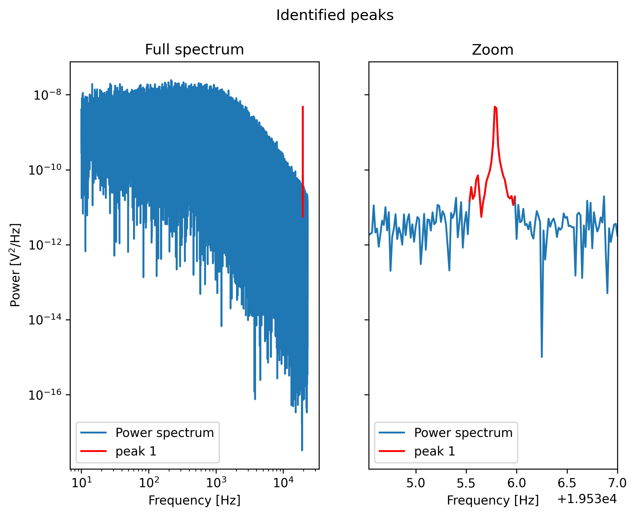We can visualize the excluded peaks as follows:

fig, ax = plt.subplots(1, 2, sharey=True)
for axis, title in zip(ax, ('Full spectrum', 'Zoom')):
    axis.loglog(ps.frequency, ps.power, label="Power spectrum")
    for idx, item in enumerate(frequency_exclusions, 1):
        to_plot = np.logical_and(item[0] <= ps.frequency, ps.frequency < item[1])
        axis.plot(ps.frequency[to_plot], ps.power[to_plot], 'r', label=f'peak {idx}')
    axis.legend()
    axis.set_title(title)
    axis.set_xlabel('Frequency [Hz]')
ax[1].set_xlim(frequency_exclusions[0][0] - 1.0, frequency_exclusions[-1][1] + 1.0)
ax[1].set_xscale('linear')
ax[0].set_ylabel('Power [V$^2$/Hz]')
plt.suptitle('Identified peaks')
plt.show()

Finally, we can do a least-squares fit, but in this case we will filter out the frequency ranges that contain peaks. Because we use a least-squares method, we get error estimates on the fit parameters, and bias in the fit result can be corrected. The default values of loss_function='gaussian' and bias_correction=True ensure least-squares fitting and bias correction, so we do not need to specify them:

ps_no_peak = lk.calculate_power_spectrum(
    f2y.data, sample_rate=f2y.sample_rate, num_points_per_block=200, fit_range=(10, 23e3), excluded_ranges=frequency_exclusions,
)
fit_no_peak = lk.fit_power_spectrum(ps_no_peak, model)

plt.figure()
fit_no_peak.plot()
plt.title(
    f"Least squares (ex. peaks): $f_c$ = {fit_no_peak.results['fc'].value:.1f}, "
    f"$D$ = {fit_no_peak.results['D'].value:.4f}, "
    f"$f_d$ = {fit_no_peak.results['f_diode'].value:.1f}"
)
plt.show()

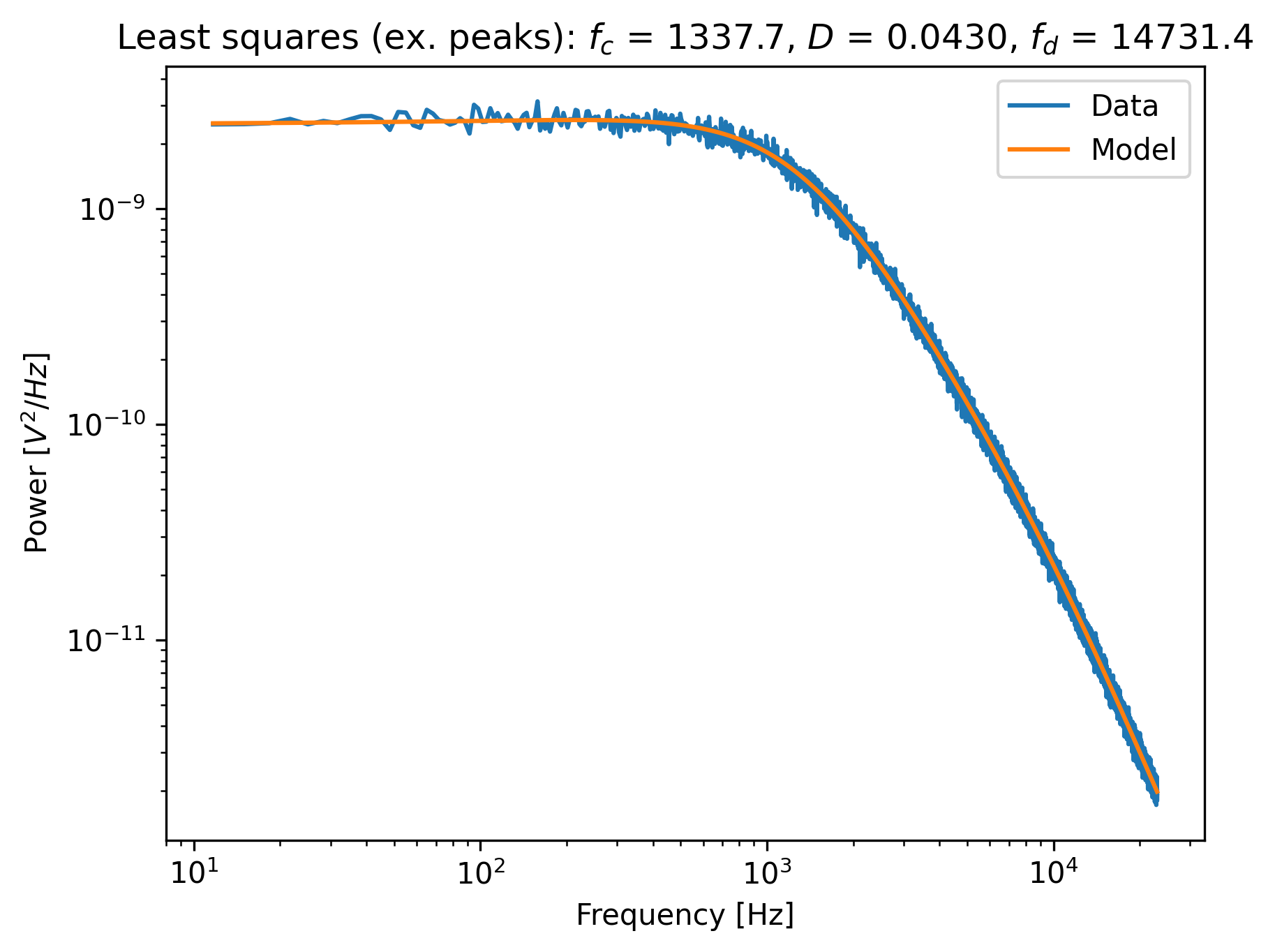
Notice that no skewing occurs, and that the values of fc, D and f_diode are now closer to values found via robust fitting in the section above.