10.3. Optimizing force calibration parameters

Download this page as a Jupyter notebook

Pylake has many options to optimize force calibration depending on the specific conditions of your experiments. The number of options presented when calling calibrate_force() may be daunting at first, but hopefully this chapter will provide some guidelines on how to obtain accurate and precise force calibrations using Pylake.

10.3.1. Experimental considerations

10.3.1.1. Core parameters

Passive calibration (also referred to as thermal calibration) involves fitting a model to data of a bead jiggling in a trap. This model relies on a number of parameters that have to be specified in order to get the correct calibration factors. The most important parameters are:

• The bead diameter (in microns).

• The viscosity of the medium, which strongly depends on temperature.

• The distance to the surface (in case of a surface experiment).

To find the viscosity of water at a particular temperature, Pylake supplies the function viscosity_of_water() which implements the model presented in [HPL+09]. When the viscosity parameter is omitted, this function will automatically be used to look up the viscosity of water for that particular temperature

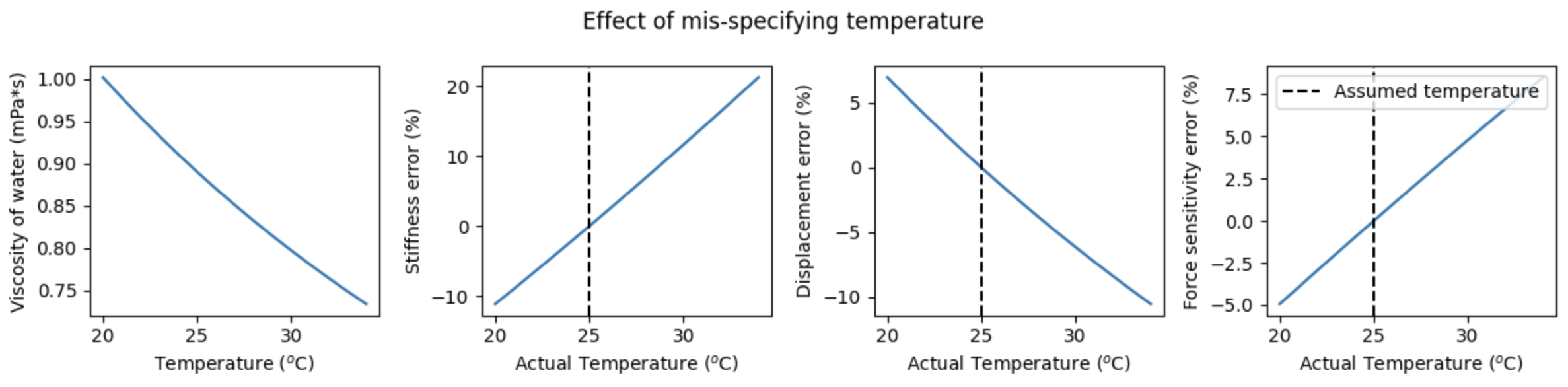
The following figure shows the effect of mis-specifying temperature on the accuracy of the (passive) calibration. The left panel shows the temperature dependence of the viscoscity of water over the expected temperature range for a typical experiment. The three right panels show the percent error expected for various calibration parameters as a function of specified temperature. The dashed vertical line indicates the actual temperature of the experiment (which corresponds to 0% error):

Note

Note that for experiments that use a medium different than water, the viscosity at the experimental temperature should explicitly be provided.

10.3.1.2. Hydrodynamically correct model

For lateral calibration, it is recommended to use the hydrodynamically correct theory by setting hydrodynamically_correct to True) as it provides an improved model of the underlying physics. For more details about this correction see the theory section on the hydrodynamically correct model. For small beads (< 1 micron) the differences will be small, but for larger beads, substantial differences can occur.

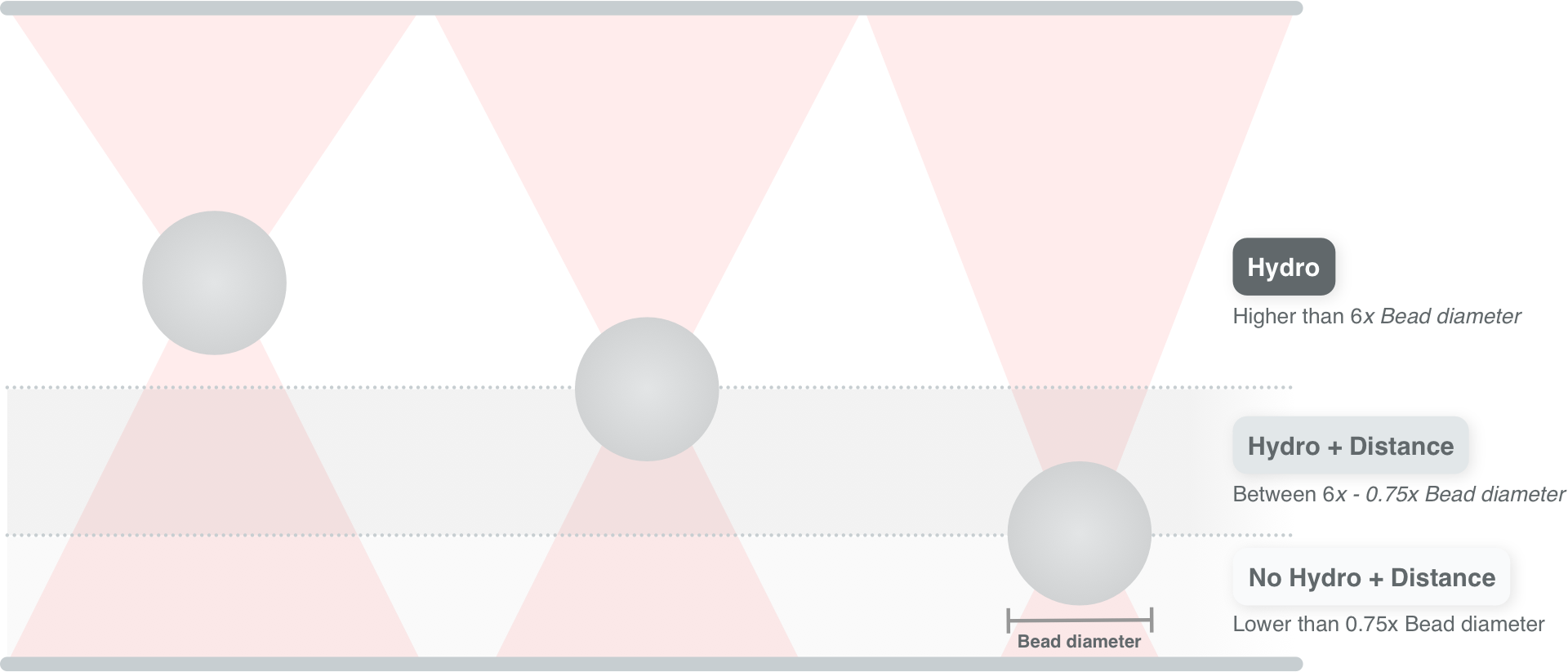
There is only one exception to this recommendation, which is when the beads are so close to the flowcell surface (0.75 x diameter) that this model becomes invalid.

Using the hydrodynamically correct theory requires a few extra parameters: the density of the sample (rho_sample) and bead (rho_bead). When these are not provided, Pylake uses values for water and polystyrene for the sample and bead density, respectively.

10.3.1.3. Experiments near the surface

Proximity of the bead to the flowcell surface leads to an increase in the drag force on the bead.

When performing experiments near the surface, it is recommended to provide the distance_to_surface argument. This should be the distance from the center of the bead to the surface of the flowcell in microns. Since it can be challenging to determine this distance, it is recommended to use active calibration when calibrating near the surface, since this makes calibration far less sensitive to mis-specification of the bead diameter, viscosity and height.

10.3.1.4. Active or passive?

Passive calibration depends strongly on the values set for the bead diameter, distance to the surface and viscosity. When these are not well known, passive calibration can be inaccurate. During active calibration, the trap or nanostage is oscillated sinusoidally, leading to additional bead motion that can be detected and used to calibrate the displacement signal. Because of this extra information, active calibration does not rely as strongly on the calibration parameters.

Active calibration is highly recommended when the bead is close to the surface, as it is less sensitive to the distance to the surface and bead diameter. It is also recommended when the viscosity of the medium or the bead diameter are poorly known. An example of a basic active calibration with a single bead can be found here.

Important

One thing to be aware of is that active calibration with two beads is more complex and currently requires manual steps in Pylake.

10.3.1.5. Axial force

When calibrating axial forces, it is important to set the axial flag to True. Note that we currently do not support hydrodynamically correct models for axial calibrations. Setting axial to True means you have to set hydrodynamically_correct to False.

10.3.2. Technical considerations

10.3.2.1. Sensor

In addition to the model that describes the bead’s motion, it is important to take into account the characteristics of the sensor used to measure the data. A silicon diode sensor is characterized by two parameters, a “relaxation factor” alpha and frequency f_diode. These parameters can either be estimated along with the other parameters or measured independently.

When the diode frequency and relaxation factor are fitted, care must be taken that the corner frequency of the power spectrum fc is lower than the estimated diode frequency. You can check whether the diode parameters were estimated from the calibration data by checking the property fitted_diode. When this property is True, it means that the diode parameters were not fixed during the fit. This means that you should be careful when calibrating small beads at high laser powers.

If the property returns False, it means you can use higher powers more safely, but will have to make sure the correct diode parameters for that particular laser power are used. For more information on how to do this, refer to the diode calibration tutorial.

Warning

For high corner frequencies, calibration can become unreliable when the diode parameters are fitted. A warning sign for this is when the corner frequency fc approaches or exceeds the diode frequency f_diode. For more information see the section on High corner frequencies.

10.3.2.2. Fit range

The fit range determines which section of the power spectrum is actually fit. Two things are important when choosing a fitting range:

1. The corner frequency should be clearly visible in the fitted range (frequency where the spectrum transitions from a plateau into a slope).

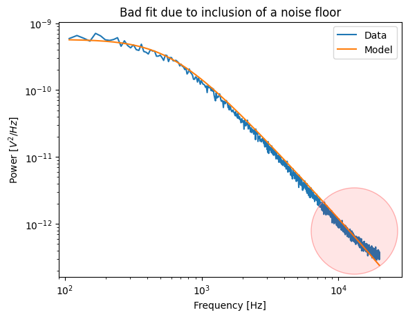
2. When working at low laser powers, it is possible that the noise floor is visible at higher frequencies. This noise floor should always be excluded from the fit.

Below is an example of a bad fit due to a noise floor. Note how the spectrum flattens out at high frequencies and the model is unable to capture this.

As a rule of thumb, an upper bound of approximately four times the corner frequency is usually a safe margin.

The fitting bounds can be specified by providing a fit_range to any of the calibration functions. When a calibrated diode is being used, they can also be determined automatically by specifying corner_frequency_factor=4 to any of the fitting functions.

10.3.2.3. Frequency exclusion ranges

Force calibration is very sensitive to outliers. It is therefore important to exclude noise peaks from the data prior to fitting. Excluding noise floors can be done by providing a list of tuples to the excluded_ranges argument of calibrate_force():

lk.download_from_doi("10.5281/zenodo.7729823", "test_data")
force_data = lk.File("test_data/robust_fit_data.h5").force2y

params = {
    "bead_diameter": 4.4,
    "temperature": 25,
    "num_points_per_block": 200,
    "hydrodynamically_correct": True,
}

calibration1 = lk.calibrate_force(
    force_data.data, sample_rate=force_data.sample_rate, **params
)
calibration2 = lk.calibrate_force(
    force_data.data, sample_rate=force_data.sample_rate, **params, excluded_ranges=[(19447, 19634)]
)

plt.figure(figsize=(8, 6))
plt.subplot(2, 2, 1)
calibration1.plot(show_excluded=True)
plt.title(f"Stiffness: {calibration1.stiffness:.3f}, Force sensi: {calibration1.displacement_sensitivity:.2f}")
plt.subplot(2, 2, 2)
calibration2.plot(show_excluded=True)
plt.tight_layout()
plt.title(f"Stiffness: {calibration2.stiffness:.3f}, Force sensi: {calibration2.displacement_sensitivity:.2f}")

plt.subplot(2, 2, 3)
calibration1.plot_spectrum_residual()
plt.ylim([0, 2])
plt.title(f"Residual\nStiffness: {calibration1.stiffness:.3f}, Force sensi: {calibration1.displacement_sensitivity:.2f}")
plt.subplot(2, 2, 4)
calibration2.plot_spectrum_residual()
plt.tight_layout()
plt.title(f"Residual\nStiffness: {calibration2.stiffness:.3f}, Force sensi: {calibration2.displacement_sensitivity:.2f}")

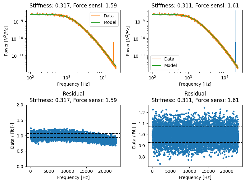
Note that when plotting the calibration, we have used show_excluded=True, which shows the excluded ranges in the plot. We can request these excluded ranges from the calibration item itself:

>>> calibration2.excluded_ranges
[(19447, 19634)]

This will also work for an item coming from Bluelake.

An alternative to specifying frequency exclusion ranges manually is robust fitting which is less sensitive to outliers. It also has an option to detect noise peaks and determine exclusion ranges automatically.

10.3.2.4. Blocking

Blocking reduces the number of points in the power spectrum by averaging adjacent points. Blocking too little means that the assumptions required to compute the statistical backing are violated and that the fit is more difficult to assess. Blocking too much can lead to a bias in the corner frequency and thereby the calibration parameters.

It is generally recommended to use more than 100 points per block. There is no clear guideline on how many points per block is too many, but a good way to check whether you are over-blocking is to change the blocking and see if it has a big impact on the corner frequency. If it does, you are likely over-blocking.

10.3.2.5. Diagnostics

Pylake offers a few diagnostics for checking whether the fit is good. Note that this in itself is not a guarantee that the calibration is correct, but it can be a good indicator whether the model curve fits the data. The first is the backing property described in more detail here. Values lower than 0.05 are generally considered suboptimal and warrant a closer inspection.

>>> calibration1.backing
0.0

>>> calibration2.backing
39.11759032609807

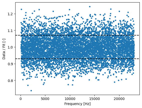
When the backing is low, it is recommended to plot the residuals of the fit. For a good fit, these should generally show a noise pattern without a clear trend such as the one below:

calibration2.plot_spectrum_residual()