Pylake 1.0.0
Pylake has made it to v1.0.0! And with it, several new features and improvements have been added.
Documentation
The documentation has been completely reworked. There is now a theory section which delves into the theory of the underlying data analysis methods, including examples and references to literature for further reading. It was split out from the tutorial section so that the tutorials can focus specifically on teaching you how to use Pylake.
Every tutorial now contains links to real C-Trap datasets hosted on Zenodo. They are downloaded as part of running the Jupyter notebooks. It simplifies trying out all the available Pylake functionality with realistic use-cases provided by the Pylake team.
Since v0.13.0, we have also reworked the API documentation to have more information on the available functions and classes in Pylake.
Creating kymographs from camera recordings
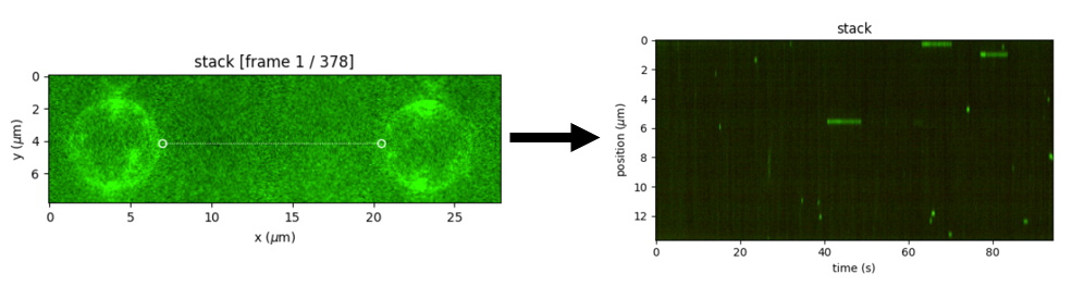
Version v1.0.0 introduces the construction of kymographs from camera recordings.
First define a tether using define_tether() which rotates the camera images such that the tether is aligned with the horizontal axis.
Then, simply call to_kymo() to sum a region around the tether and construct a Kymo.
To read more about this feature, please refer to the tutorial.
Bias correction
When tracking kymographs, the default refinement algorithm used to achieve sub-pixel localization accuracy is based on centroid refinement.
Centroid refinement can suffer from bias (tending towards the pixel center) when there is considerable background in the image.
Pylake v1.0.0 removes this bias using the method presented in [BMML08].
For best results, we recommend using gaussian refinement after tracking.

Localization in the presence of high background. On the x-axis is the true position of a fluorescent spot, while on the y-axis, we see its inferred location. From left to right: regular centroid refinement, bias-corrected refinement and Gaussian refinement. From top to bottom: The top row shows localization performed with a small window, while the bottom row shows localization performed with a large window. The step-like progression in the centroid case is due to the bias induced by the background intensity. These steps originate from a bias towards the center of each pixel. Note how the bias corrected variant more closely agrees with the Gaussian refinement result. For Gaussian refinement, a larger window is beneficial (as it uses more data and models the background), while for centroid refinement it can lead to a larger estimation variance because of the inclusion of more noise.
Scalebars
With Pylake v1.0.0 you can add scale bars to just about any image plot by simply including a scale_bar=lk.ScaleBar() argument to .plot() or .export_video().
See ScaleBar for more information.

Movie exported from Pylake with scan.export_video("rgb", "scan_stack.gif", scale_bar=lk.ScaleBar())).
Calibrated Images
Camera images now show the image in microns rather than pixels.

Other changes
Since this is a major release, it includes breaking changes. Note that we adhere to semantic versioning, meaning that we increment the major version number to indicate that there are breaking changes. As always, we implemented various other bug-fixes and improvements.
For a full list of all the changes, please refer to the full changelog.
Happy Pylake-ing!