11. Population Dynamics
Download this page as a Jupyter notebook
The following tools enable analysis of experiments which can be described as a system of discrete states. Consider as an example a DNA hairpin which can exist in a folded and unfolded state. At equilibrium, the relative populations of the two states are governed by the interconversion kinetics described by the rate constants \(k_\mathrm{fold}\) and \(k_\mathrm{unfold}\)
We can download the data needed for this tutorial directly from Zenodo using Pylake.
Since we don’t want it in our working folder, we’ll put it in a folder called "test_data":
filenames = lk.download_from_doi("10.5281/zenodo.7729812", "test_data")
First let’s take a look at some example force channel data. We’ll downsample the data in order to speed up the calculations and smooth some of the noise:
file = lk.File("test_data/hairpin.h5")
raw_force = file.force2x
force = raw_force.downsampled_by(78)

plt.figure()
raw_force.plot()
force.plot(start=raw_force.start)
plt.xlim(0, 2)  # let's zoom to the first 2 seconds
plt.show()
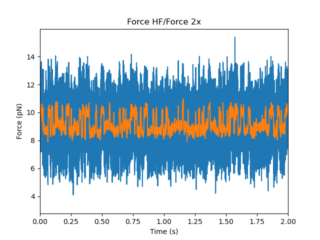
Care must be taken in downsampling the data so as not to introduce signal artifacts in the data (see below for a more detailed discussion).
The goal of the analyses described below is to label each data point in a state in order to extract kinetic and thermodynamic information about the underlying system.
11.1. Gaussian Mixture Models
The Gaussian Mixture Model (GMM) is a simple probabilistic model that assumes all data points belong to one of a fixed number of states (\(K\)), each of which is described by a normal distribution \(\mathcal{N}(\mu, \sigma)\) weighted by some factor \(\phi\). The probability distribution function of this model is
The weights \(\phi_i\) give the fraction of time spent in each state with the constraint \(\sum_i^K \phi_i = 1\). The means \(\mu_i\) and standard deviations \(\sigma_i\) indicate the average signal and noise for each state, respectively.
The Pylake GMM implementation GaussianMixtureModel is a wrapper around sklearn.mixture.GaussianMixture with some
added convenience methods and properties for working with C-Trap data.
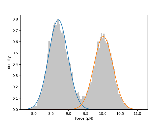
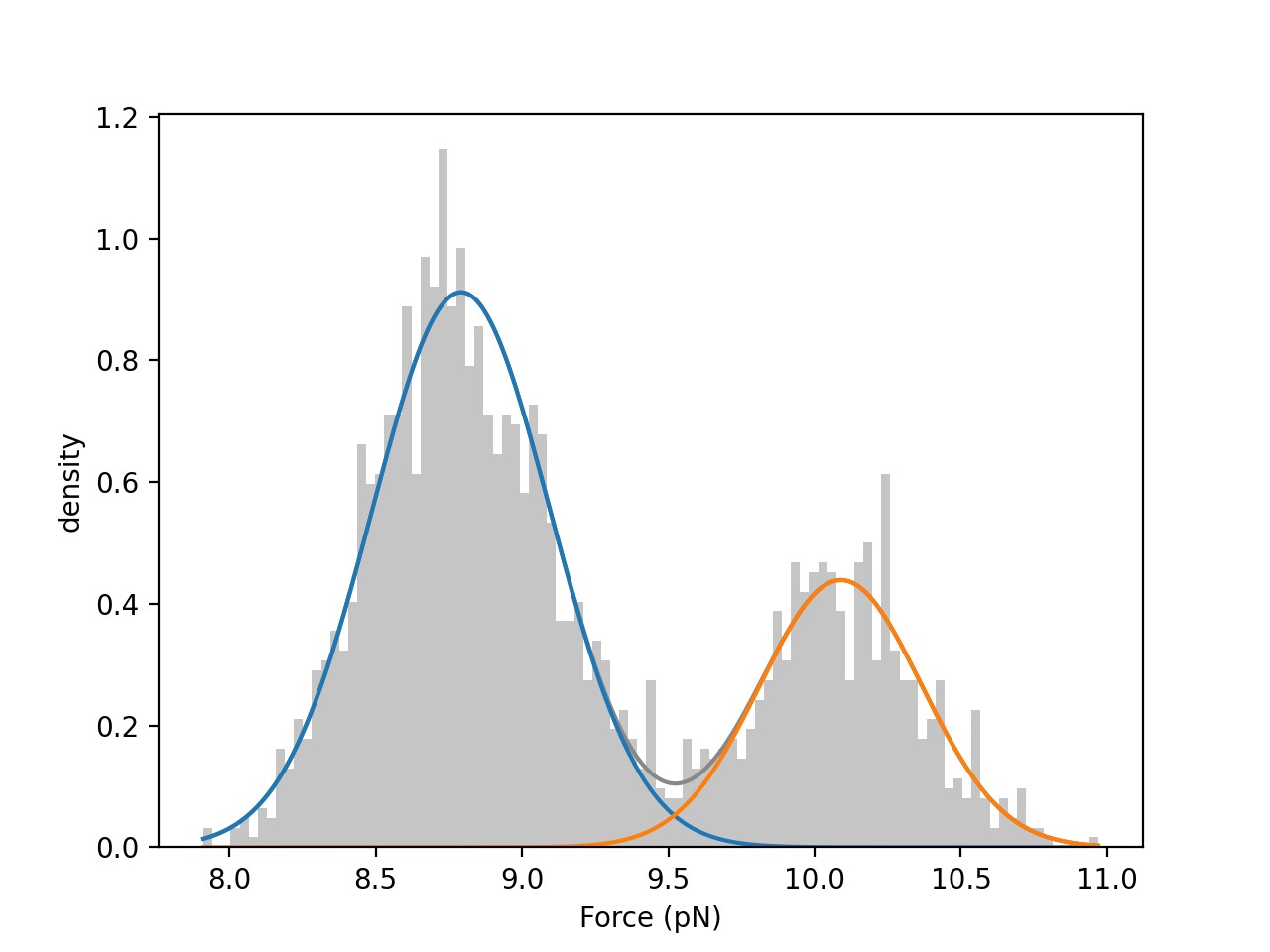
Here we train a two-state model using only the first 20 seconds of the force data to speed up the calculation:
gmm = lk.GaussianMixtureModel(force["0s":"20s"], n_states=2)
We can inspect the parameters of the model with the weights, means,
and std properties. Note that, unlike the scikit-learn implementation, the states here are always ordered from
smallest to largest mean value:
print(gmm.weights)  # [0.55505362 0.44494638]
print(gmm.means)  # [8.70803166 10.01637358]
print(gmm.std)  # [0.27888473 0.27492966]
Note
Note, in the following examples we do not have to use the same slice of data that was used to train the model; once a model is trained, it can be used to infer the states from any data that is properly described by it.
A common strategy to minimize the amount of time spent on training the model is to do precisely what we did here – train with only a small fraction of the data and then use the trained model to infer results about the full dataset. This approach is only valid, however, if the training data fully captures the behavior of the full dataset. It is good practice to inspect the histogram with the full data or a larger slice of the data than was used to train the model to check the validity of the optimized parameters.
We can visually inspect the quality of the fitted model by plotting a histogram of the data overlaid with the weighted normal distribution probability density functions:
plt.figure()
gmm.hist(force["0s":"20s"])
plt.show()
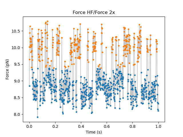
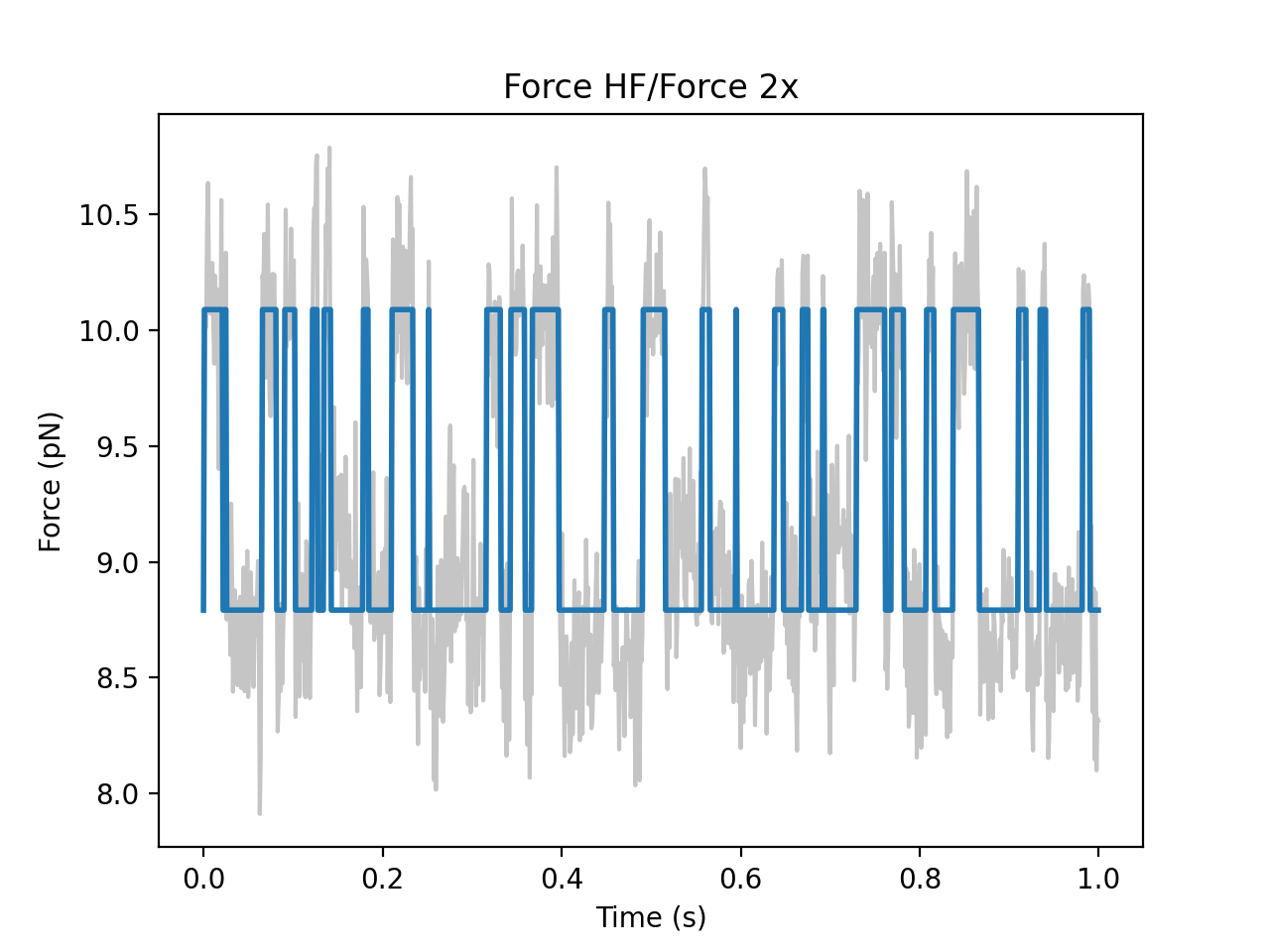
We can also plot the time trace with each data point labeled with its most likely state:
plt.figure()
gmm.plot(force['0s':'1s'])
plt.show()
11.1.1. Downsampling and data artifacts
As mentioned before, it can be desirable to downsample the raw channel data in order to decrease the number of data points used by the model training algorithm (in order to speed up the calculation) and to smooth experimental noise. However, great care must be taken in doing so in order to avoid introducing artifacts in the signal.
We can test this by training models on the same data downsampled by different factors:
plt.figure()

for j, ds_factor in enumerate([10, 78, 350]):
    plt.subplot(3, 1, j+1)
    ds = raw_force["0s":"20s"].downsampled_by(ds_factor)
    tmp_gmm = lk.GaussianMixtureModel(ds, n_states=2)
    tmp_gmm.hist(ds)
    plt.xlim(8, 11)
    plt.title(f"downsampled by {ds_factor}")

plt.tight_layout()
plt.show()
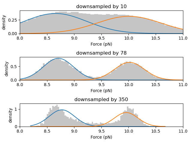
As shown in the histograms above, as the data is downsampled the state peaks narrow considerably, but density between the peaks remains. These intermediate data points are the result of averaging over a span of data from two different states and do not arise from any (bio)physically relevant mechanism.
Furthermore, states with very short lifetimes can be averaged out of the data if the downsampling factor is too high. Therefore, in order to ensure robust results, it may be advisable to carry out the analysis at a few different downsampled rates.
11.3. Dwell time analysis
The lifetimes of bound states can be estimated by fitting observed dwell times \(t\) to a mixture of Exponential distributions.
where each of the \(M\) exponential components is characterized by a lifetime \(\tau_i\) and an amplitude (or fractional contribution) \(a_i\) under the constraint \(\sum_i a_i = 1\). The lifetime describes the mean time a state is expected to persist before transitioning to another state. The distribution can alternatively be parameterized by a rate constant \(k_i = 1 / \tau_i\).
The DwelltimeModel class can be used to optimize the model parameters for an array
of determined dwell times (how long the system stays in one state before transitioning to another).
We can extract arrays of dwell times for all states in a GMM or HMM with
lk.GaussianMixtureModel.extract_dwell_times()
or lk.HiddenMarkovModel.extract_dwell_times(),
respectively:
dwell_times = gmm.extract_dwell_times(force)
This returns a dictionary with state indices as keys and lists of the observed dwell times as the values.
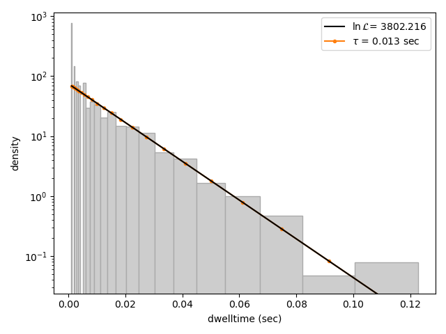
We can fit a model by passing the array of dwell times to DwelltimeModel:
dwell_1 = lk.DwelltimeModel(dwell_times[1], n_components=1)
The model is optimized using Maximum Likelihood Estimation (MLE) [KJC+19, WLG+16]. The advantage of this method
is that it does not require binning the data. The number of exponential components to be used for the fit is chosen with the n_components argument.
The optimized model parameters can be accessed with the lifetimes and amplitudes
properties. In the case of first order kinetics, the rate constants can be accessed with the rate_constants property.
This value is simply the inverse of the optimized lifetime(s). See Discretization for more information.
We can visually inspect the result with:
plt.figure()
dwell_1.hist(bin_spacing="log")
plt.show()
The bin_spacing argument can be either "log" or "linear" and controls the spacing of the bin edges.
The scale of the x- and y-axes can be controlled with the optional xscale and yscale arguments; if they are not specified
the default visualization is lin-lin for bin_spacing="linear" and lin-log for bin_spacing="log". You can also optionally pass the number of
bins to be plotted as n_bins.
Note
The number of bins is purely for visualization purposes; the model is optimized directly on the unbinned dwell times. This is the main advantage of the MLE method over analyses that use a least squares fitting to binned data, where the bin widths and number of bins can drastically affect the optimized parameters.
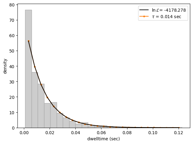
This distribution seems to be fit well with a single exponential component, however there is some density at short dwell times that is missed. We can also try a double exponential fit to see if the fitting improves:
dwell_2 = lk.DwelltimeModel(dwell_times[1], n_components=2)

plt.figure()
dwell_2.hist(bin_spacing="log")
plt.show()
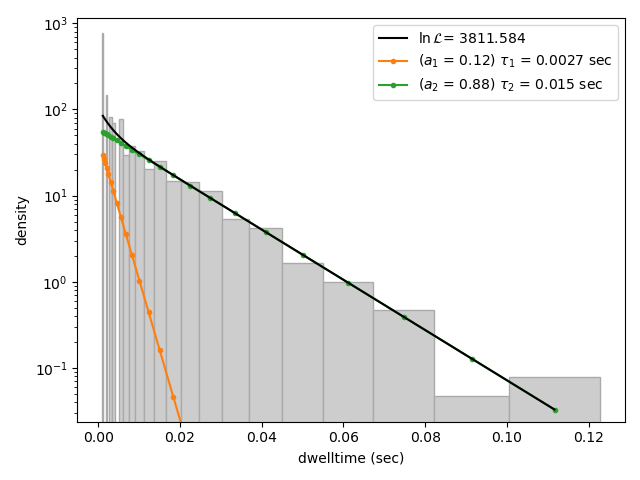
Here we see visually that there is no significant improvement in the quality of the fit, so the single exponential is probably a better model for these data.
We can also use some statistics to help choose the most appropriate model. The MLE method maximizes a likelihood function, with the final value reported in the legend of the histogram. We see that the likelihood of the double exponential model is slightly higher than that of the single exponential model which might suggest that the double exponential model is better. However, the likelihood does not take into account model complexity and will always increase with increasing number of adjustable parameters.
More informative statistics for model comparison are the Information Criteria. Two specific criteria are available from the model: the Bayesian Information Criterion (BIC) and the Akaike Information Criterion (AIC):
print(dwell_1.bic, dwell_1.aic)  # -7597.384625071581 -7602.4312723494295
print(dwell_2.bic, dwell_2.aic)  # -7602.027247179558 -7617.167189013104
These information criteria values weigh the log likelihood against the model complexity, and as such are more useful for model selection. In general, the model with the lowest value is optimal. We can see that both values are lower for the double exponential model, but only slightly so it is not strong evidence to choose the more complex model.
11.3.1. Standard errors
After the optimal model for the data has been selected using the methods above, the reliability of the parameter estimates can be determined.
Pylake provides several methods to determine both the confidence intervals and the standard errors of the parameters.
For large datasets, the standard error under err_amplitudes and err_lifetimes can be used. Note that these are only asymptotically correct:
>>> dwell_1.err_lifetimes
array([0.00039664])
>>> dwell_2.err_amplitudes
array([0.03601527, 0.03601527])
>>> dwell_2.err_lifetimes
array([0.00072262, 0.00063035])
In most cases, what we would actually like to have are confidence intervals. If we were to repeat the experiment many times, the true parameter would fall inside the confidence interval a set fraction of the time (confidence level). We can convert these asymptotic standard errors into confidence intervals (CI) using the \(\chi^2\) distribution:
def to_ci(parameter_value, std_err, confidence_level):
    import scipy

    chi_squared = scipy.stats.chi2.ppf(confidence_level, 1)
    d = np.sqrt(chi_squared * std_err ** 2)
    return [parameter_value - d, parameter_value + d]
For example, to get the 95% confidence interval for dwell time 2, we could invoke:
>>> print(to_ci(dwell_2.lifetimes[1], dwell_2.err_lifetimes[1], 0.95))
[0.01486646499028639, 0.014945519089580198]
For more rigorous uncertainty analysis, consider the options below.
11.3.2. Confidence intervals from bootstrapping
As an additional check, we can estimate confidence intervals (CI) for the parameters using bootstrapping. Here, a dataset with the same size as the original is randomly sampled (with replacement) from the original dataset. This random sample is then fit using the MLE method, just as for the original dataset. The fit results in a new estimate for the model parameters. This process is repeated many times, and the distribution of the resulting parameters can be analyzed to estimate certain statistics about them.
We can calculate a bootstrap distribution with calculate_bootstrap():
bootstrap_2 = dwell_2.calculate_bootstrap(iterations=100)

plt.figure()
bootstrap_2.hist(alpha=0.05)
plt.show()
Here we see the distributions of the bootstrapped parameters, each of which ideally should look like a Normal (Gaussian) distribution.
The vertical lines indicate the means of the distributions, while the red area indicates the estimated confidence intervals.
The alpha argument determines the CI that is estimated as 100*(1-alpha) % CI; in this case we’re showing the estimate for the 95% CI.
The values for the lower and upper bounds are the 100*(alpha/2) and 100*(1-alpha/2) percentiles of the distributions.
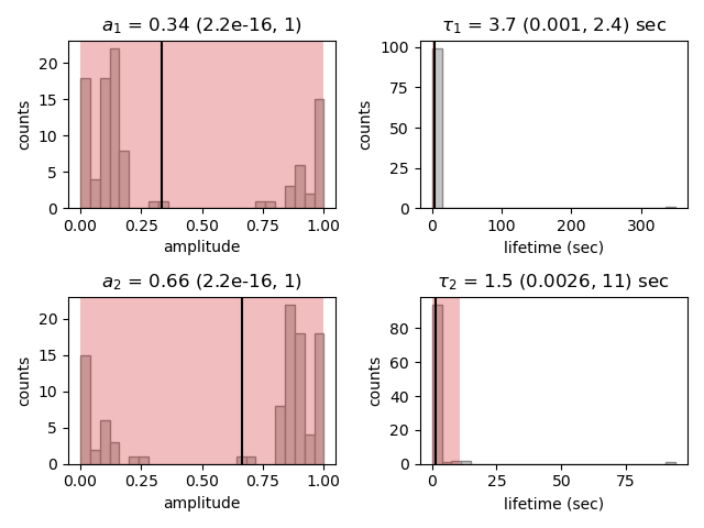
Clearly the distributions here are not Gaussian. Specifically, the two distributions on the left for the fractional amplitudes are split. In fact, many amplitudes are estimated near zero which effectively removes that component from the model. This analysis strongly indicates that the single exponential model is preferable. We can also look at the bootstrap for that model to verify the results are satisfactory:
bootstrap_1 = dwell_1.calculate_bootstrap(iterations=100)

plt.figure()
bootstrap_1.hist(alpha=0.05)
plt.show()
Here we only see one distribution since the fractional amplitude for a single exponential model is 1 by definition. The results
look much better, with most of the distribution being fairly Gaussian with the exception of some outliers at longer lifetimes.
These likely are the result of poorly fit or numerical unstable models.
Note
As we have seen, care must be taken when choosing between different models and interpreting the bootstrapped confidence intervals. The means of the bootstrap distribution should correspond well with the optimized model parameters from the original data. Here, we only ran 100 iterations of the sampling to keep the analysis time short for exploratory purposes. When computing the distributions to obtain final values when a model has been selected, you should generally run significantly more iterations.
As mentioned before, ideally the bootstrapped distributions should also be normally distributed. However sometimes even
valid models can yield skewed distributions. In such a case, the simple method of using percentiles as CI values may not be appropriate.
For more advanced analysis, the distribution values are directly available through the properties
amplitude_distributions
and lifetime_distributions which return the data as a numpy array with
shape [# components, # bootstrap samples].
11.3.3. Speeding up bootstraps
Models with a larger number of components typically require more bootstrap samples to adequately characterize their uncertainty histograms. Consequently, the bootstrapping process can become quite time consuming.
To accelerate this process, you can use the num_processes argument in the calculate_bootstrap() method:
import psutil

# A good number of processes to choose is the number of physical cores in the system
cpu_count = psutil.cpu_count(logical=False)
bootstrap_parallel = dwell_1.calculate_bootstrap(iterations=100, num_processes=cpu_count)
11.3.4. Profile Likelihood based Confidence intervals
We also offer a deterministic method for estimating confidence intervals.
This method is known as the profile likelihood method [MHS+16, RKM+09] and is described in more detail here.
Profile likelihood can be applied for model selection as it tests whether the data can be fit with fewer parameters without a reduction in fit quality.
It can be invoked by calling lumicks.pylake.DwelltimeModel.profile_likelihood():
profiles = dwell_2.profile_likelihood()

plt.figure()
profiles.plot(with_stderr=True)
plt.tight_layout()
plt.show()
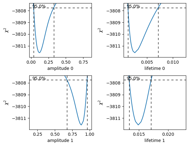
The intersection points between the blue curve and the dashed horizontal lines indicate the confidence interval.
Here, we called it with with_stderr so we can see how the profiles compare to the asymptotic results (see also Standard errors) which are shown with dashed lines.
These can be extracted by using the get_interval() method from the DwelltimeProfiles:
>>> # Get confidence intervals
... for component in range(2):
...     interval = profiles.get_interval("amplitude", component)
...     print(f"Amplitude {component}: {interval}")
...     interval = profiles.get_interval("lifetime", component)
...     print(f"Lifetime {component}: {interval}")
Amplitude 0: (0.05982816424650479, 0.21741436565540087)
Lifetime 0: (0.001636984107953483, 0.004916100332753989)
Amplitude 1: (0.7825797139037362, 0.9401719367915693)
Lifetime 1: (0.013775669029270098, 0.016306865025599655)
If the confidence interval for any of the amplitudes contains zero, then that component contributes very little to the model fit and a model with fewer components should be used.
11.3.5. Discretization
While the kinetic processes being analyzed are continuous, the observed dwell times are measured at discrete intervals (multiples of the sampling rate).
When lifetimes are short compared to the sampling rate this can have an effect on the parameter estimates.
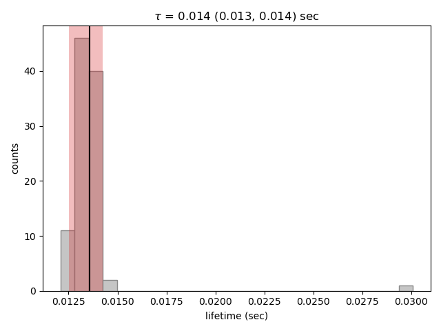
To take the discretization into account, we can provide a time step to the DwelltimeModel:
dwell_d = lk.DwelltimeModel(
    dwell_times[1],
    n_components=1,
    discretization_timestep=1.0/force.sample_rate,
    min_observation_time=1.0/force.sample_rate,
)

plt.figure()
dwell_d.hist()
plt.show()
As we can see, the difference in this case is small, but the effect of discretization can be more prominent when lifetimes approach the sampling time.
11.3.6. Assumptions and limitations on determining rate constants
When using an exponential distribution to model biochemical kinetics, care must be taken to ensure that the model appropriately describes the observed system. Here we briefly describe the underlying assumptions and limitations for using this method.
The exponential distribution describes the expected dwell times for states in a first order reaction where the rate of transitioning from the state is dependent on the concentration of a single component. A common example of this is the dissociation of a bound protein from a DNA strand:
This reaction is characterized by a rate constant \(k_\mathrm{off}\) known as the dissociation rate constant with units of \(\mathrm{sec}^{-1}\).
Second order reactions which are dependent on two reactants can also be determined in this way if certain conditions are met. Specifically, if the concentration of one reactant is much greater than that of the other, we can apply the first order approximation. This approximation assumes the concentration of the more abundant reactant remains approximately constant throughout the experiment and therefore does not contribute to the reaction rate. This condition is often met in single-molecule experiments; for example in a typical C-Trap experiment, the concentration of a protein in solution on the order of nM is significantly higher than the concentration of the single trapped tether.
A common example of this is the binding of a protein to a DNA strand:
This reaction is described by the second order association rate constant \(k_\mathrm{on}\) with units of \(\mathrm{M}^{-1}\mathrm{sec}^{-1}\). Under the first order approximation, this can be determined by fitting the appropriate dwell times to the exponential model and dividing the resulting rate constant by the concentration of the protein in solution.
Note
The calculation of \(k_\mathrm{on}\) relies on having an accurate measurement of the bulk concentration. Care should be taken as this can be difficult to determine when working in the nanomolar regime, as nonspecific adsorption can lower the effective concentration at the experiment.
11.3.7. A warning on reliability and interpretation of multi-exponential kinetics
Sometimes a process can best be described by two or more exponential distributions. This occurs when a system consists of multiple states with different kinetics that emit the same observable signal. For instance, the dissociation rate of a bound protein might depend on the microscopic conformation of the molecule that does not affect the emission intensity of an attached fluorophore used for tracking. Care must be taken when interpreting results from a mixture of exponential distributions.
However, in the setting of a limited number of observations, the optimization of the exponential mixture can become non-identifiable, meaning that there are multiple sets of parameters that result in near equal likelihoods. A good first check on the quality of the optimization is to run a bootstrap simulation (as described above) and check the shape of the resulting distributions. Very wide, flat, or skewed distributions can indicate that the model was not fitted to a sufficient amount of data. For processes that are best described by two exponentials, it may be necessary to acquire more data to obtain a reliable fit.
11.3.8. The Exponential (Mixture) Model
The model likelihood \(\mathcal{L}\) to be maximized is defined for a mixture of exponential distributions as:
where \(T\) is the number of observed dwell times, \(M\) is the number of exponential components, \(t\) is time, \(\tau_i\) is the lifetime of component \(i\), and \(a_i\) is the fractional contribution of component \(i\) under the constraint of \(\sum_i^M a_i = 1\). The normalization constant \(N\) is defined as:
where \(t_{min}\) and \(t_{max}\) are the minimum and maximum possible observation times.
The normalization constant takes into account the minimum and maximum possible observation times of the experiment. These
can be set manually with the min_observation_time and max_observation_time keyword arguments, respectively. The default
values are \(t_{min}=0\) and \(t_{max}=\infty\), such that \(N=1\). However, for real experimental data,
there are physical limitations on the measurement times (such as pixel integration time for kymographs or sampling frequency for
force channels) that should be taken into account.
11.3.9. Discrete model
While it is tempting to discretize the exponential distribution directly, this would not give correct results. The start and end point of a dwell are discrete multiples of the acquisition rate; these are the values which are discretized. Consider the probability density of a dwell starting uniformly over the sampling interval. The probability density that an event is captured at dwell time \(f \Delta t\) is given by a triangular probability from \(t = (f - 1)\Delta t\) to \(t = (f + 1)\Delta t\) [LJW+17], where \(f\) is the frame index and \(\Delta t\) the sampling interval. We can simulate this:
n_samples = 5000
probability = []
positions = np.arange(0, 4, 0.01)
for true_dwell in positions:
    start_pos = np.random.rand(n_samples)
    end_pos = start_pos + true_dwell
    correct = (np.floor(end_pos) - np.floor(start_pos)) == 2
    probability.append(np.sum(correct) / n_samples)

plt.plot(positions, probability)
plt.ylabel(f'Probability of being sampled at t=2')
plt.xlabel('True dwell time [s]')
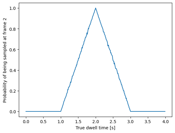
This means that if we want to know the probability of observing a particular dwell duration (in whole frames), we need to multiply the probability density of the dwell time model by this observation model and then integrate it. Discretization of the continuous model with discretization time step \(\Delta t\) then amounts to evaluating the following integrals:
Given that
and
we obtain
or
To take into account the finite support (minimum and maximum dwelltime), we have to renormalize the distribution to the minimum and maximum frame.
The normalization constant \(N_j\) is given by:
The sum is a geometric series and evaluates to:
Considering that:
we can see that part of the denominator will cancel out. This evaluates to the following expression:
or (in a more similar form as the continuous case)
for the normalization constant of a particular data point.