2. FD Curves
Download this page as a Jupyter notebook
We can download the data needed for this tutorial directly from Zenodo using Pylake.
Since we don’t want it in our working folder, we’ll put it in a folder called "test_data":
filenames = lk.download_from_doi("10.5281/zenodo.7729929", "test_data")
Once we have the data, we can load the HDF5 file and list all FD curves inside the file:
>>> file = lk.File("test_data/fdcurve.h5")
>>> list(file.fdcurves)
['FD_5_control_forw']
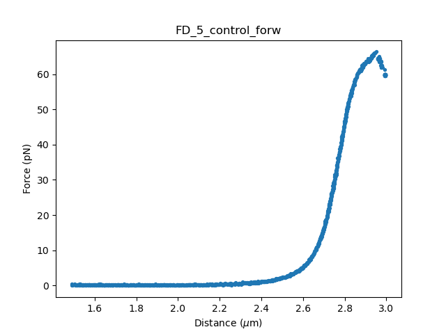
To visualizes an FD curve, you can use the built-in .plot_scatter() method:
plt.figure()
fd = file.fdcurves["FD_5_control_forw"]
fd.plot_scatter()
plt.show()
An FdCurve slices some force and distance data from the timeline data.
You can find the range it uses for slicing in its start and stop property:
>>> all(file.downsampled_force2[fd.start : fd.stop].data == fd.f.data)
True
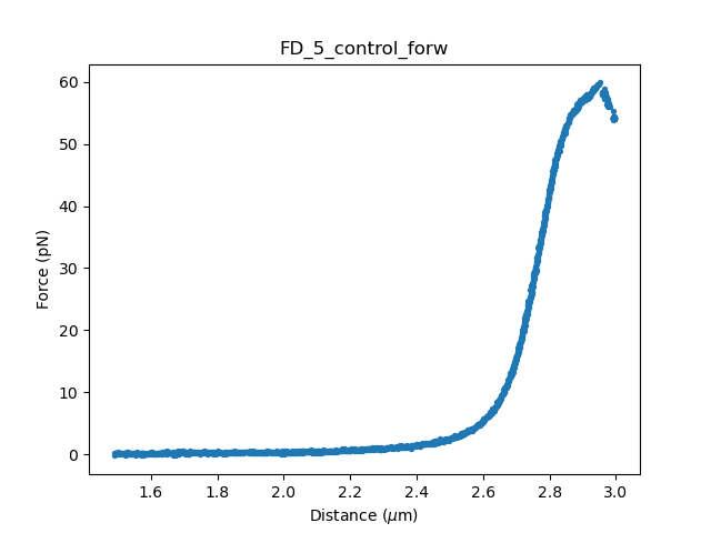
The attribute .fdcurves is a standard Python dictionary, so we can do all the things you can do with a regular dictionary.
For example, we can iterate over all the FD curves in a file and plot them:
plt.figure()
for name, fd in file.fdcurves.items():
    fd.plot_scatter()
plt.show()
By default, the FD channel pair is downsampled_force2 and distance1.
This assumes that the force extension was done by moving trap 1, which is the most common.
In that situation the force measured by trap 2 is more precise because that trap is static.
Note
The default force channel used by an FdCurve is downsampled_force2.
Channel names without a suffix represent a total force, e.g. \(\sqrt{F_{2, x}^2 + F_{2, y}^2}\).
The channels can be switched with the following code:
plt.figure()
alt_fd = fd.with_channels(force='1x', distance='1')
alt_fd.plot_scatter()
plt.show()
or as quick one-liner for plotting:
plt.figure()
fd.with_channels(force='1x', distance='1').plot_scatter()
plt.show()
Other force channels that can be selected are '1y' and '2y' and the distance channel can also have value '2'.
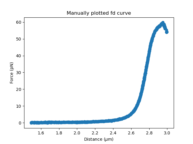
The raw data can be accessed as well:
# Access the raw data: default force and distance channels
force = fd.f
distance = fd.d

# Access the raw data: specific channels
force = fd.downsampled_force1x
distance = fd.distance1
Plot FD curve manually:
plt.figure()
plt.scatter(distance.data, force.data)
plt.ylabel("Force (pN)")
plt.xlabel(r"Distance ($\mu$m)")
plt.title("Manually plotted fd curve")
plt.show()
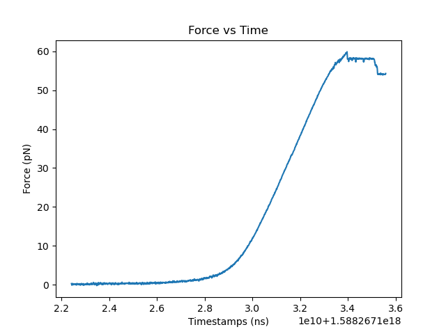
Plot force versus time manually:
plt.figure()
plt.plot(force.timestamps,force.data)
plt.ylabel("Force (pN)")
plt.xlabel("Timestamps (ns)")
plt.title("Force vs Time")
plt.show()
2.1. FD Ensembles
FD curves can be aligned by combining them in an FdEnsemble.
If all the fd curves of interest are in the same file, the ensemble can be defined as
fd_ensemble = lk.FdEnsemble(ensemble_file.fdcurves). If the fd curves are in different files, the ensemble can be defined as follows:
ensemble_file1 = lk.File("test_data/fd_hairpin_fwd.h5")
ensemble_file2 = lk.File("test_data/fd_hairpin_back.h5")
fd_ensemble = lk.FdEnsemble({**ensemble_file1.fdcurves,**ensemble_file2.fdcurves})
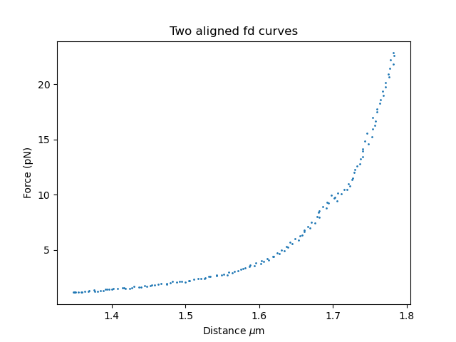
We can align the FD curves using the align function:
fd_ensemble.align_linear(distance_range_low=0.02, distance_range_high=0.02)
This aligns all the curves to the first and estimates an offset in force and distance, which is subtracted from the data. Force is aligned by taking the mean of the lowest distances, while distance is aligned by considering the last segment of each FD curve and regressing linear lines there, from which the offset is computed. Note that this requires the ends of the aligned F,d curves to be in a comparably folded state and obtained in the elastic range of the force, distance curve. If any of these assumptions are not met, this method should not be applied. We can obtain the force and distance from such an ensemble using:
f = fd_ensemble.f
d = fd_ensemble.d

plt.figure()
plt.scatter(d, f, s=1)
plt.ylabel("Force (pN)")
plt.xlabel(r"Distance $\mu$m")
plt.title("Two aligned fd curves")
plt.show()
2.2. Baseline Correction
FD curves can also be constructed from baseline corrected force data using with_baseline_corrected_x()
if the channel was exported from Bluelake with a baseline correction applied.
Note
By default, FD curves are constructed using the force magnitude \(F = \sqrt{F_x^2 + F_y^2}\). However, baseline correction in Bluelake is only calculated for the x-component \(F_x\). Therefore, FD curves with baseline correction applied are constructed with only the x-component rather than the full magnitude and may not be directly comparable to the corresponding uncorrected FD curve.
Additionally, baseline-corrected FD curves are read directly from the source HDF5 file. Therefore, any data processing previously applied to the FD curve used to obtain the baseline corrected curve is lost.