1. Files and Channels
Download this page as a Jupyter notebook
We can download the data needed for this tutorial directly from Zenodo using Pylake.
Since we don’t want it in our working folder, we’ll put it in a folder called "test_data":
filenames = lk.download_from_doi("10.5281/zenodo.7729525", "test_data")
Once we have the data, we can open the Bluelake HDF5 file as follows:
import lumicks.pylake as lk

file = lk.File("test_data/kymo.h5")
1.1. Contents
To see a textual representation of the contents of a file:
>>> print(file)
File root metadata:
- Bluelake version: experimental/workflows-1
- Description:
- Experiment:
- Export time (ns): 1638534716503544400
- File format version: 2
- GUID: {3187B298-AF67-477C-98D0-CF176808E995}

Bead diameter:
  Template 1:
  - Data type: [('Timestamp', '<i8'), ('Value', '<f8')]
  - Size: 3151
  Template 2:
  - Data type: [('Timestamp', '<i8'), ('Value', '<f8')]
  - Size: 3151
Confocal diagnostics:
  Excitation Laser Blue:
  - Data type: [('Timestamp', '<i8'), ('Value', '<f8')]
  - Size: 1
  Excitation Laser Green:
  - Data type: [('Timestamp', '<i8'), ('Value', '<f8')]
  - Size: 3
  Excitation Laser Red:
  - Data type: [('Timestamp', '<i8'), ('Value', '<f8')]
  - Size: 3
Distance:
  Distance 1:
  - Data type: [('Timestamp', '<i8'), ('Value', '<f8')]
  - Size: 3151
Force HF:
  Force 1x:
  - Data type: float64
  - Size: 16405001
  Force 1y:
  - Data type: float64
  - Size: 16405001
  Force 2x:
  - Data type: float64
  - Size: 16405001
  Force 2y:
  - Data type: float64
  - Size: 16405001
Info wave:
  Info wave:
  - Data type: uint8
  - Size: 16405001
Note
Other
Photon count:
  Blue:
  - Data type: uint32
  - Size: 16405001
  Green:
  - Data type: uint32
  - Size: 16405001
  Red:
  - Data type: uint32
  - Size: 16405001
Piezo Calibration
Point Scan

.markers
  - Tether: 11

.kymos
  - 16

.force1x
  .calibration
.force1y
  .calibration
.force2x
  .calibration
.force2y
  .calibration
Listing specific timeline items:
>>> list(file.markers)
['Tether: 11']

>>> list(file.kymos)
['16']
They can also be printed to get more information:
>>> print(file.kymos)
{'16': Kymo(pixels=699)}
1.2. Channels
Just like the Bluelake timeline, exported HDF5 files contain multiple channels of data.
They can be accessed as file[group name][channel name], where the group and channel name can be found in Bluelake, or using the print(file) statement, for example:
file['Force HF']['Force 1x']
All channel data can be accessed using the above method. High frequency force data can also be accessed as:
file.force1x
The only difference between the two above methods for accessing channel data, is that file.force1x allows you to access the force calibration data, as described below.
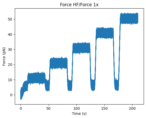
Plotting the data can be done as follows:
plt.figure()
file.force1x.plot()
plt.savefig("force1x.png")
plt.show()

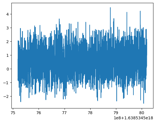
You can also access the raw data directly:
f1x_data = file.force1x.data
f1x_timestamps = file.force1x.timestamps

plt.figure()
plt.plot(f1x_timestamps, f1x_data)
plt.show()
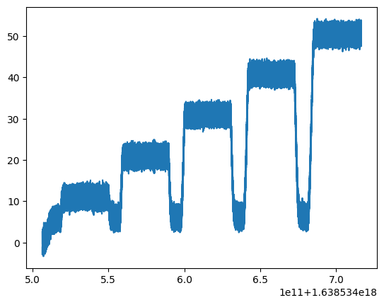
The timestamps attribute returns the measurement time in nanoseconds since epoch (January 1st 1970, midnight UTC/GMT). Note that since these values are typically very large, they cannot be converted to floating point without losing precision:
>>> t = f1x_timestamps[0]
>>> roundtrip_t = np.int64(np.float64(t))
>>> print(t - roundtrip_t)
80
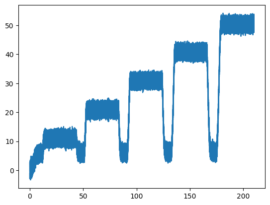
The relative time values in seconds can also be accessed directly:
f1x_seconds = file.force1x.seconds

plt.figure()
plt.plot(f1x_seconds, f1x_data)
plt.show()
A full list of available channels can be found on the File reference page.
1.2.1. Slicing
By default, entire channels are returned from a file:
everything = file.force1x

plt.figure()
everything.plot()
plt.show()
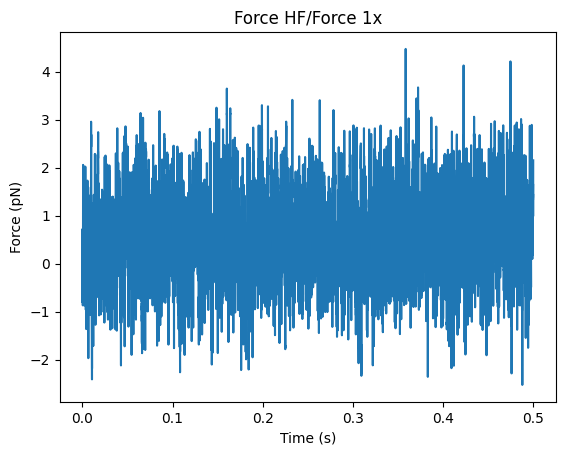
But channels can also be sliced:
# Get the data between 1 and 1.5 seconds and use the plot function in Pylake
part = file.force1x['1s':'1.5s']

plt.figure()
part.plot()
plt.show()
# Access the raw data and plot using matplotlib
f1x_data = part.data
f1x_timestamps = part.timestamps

plt.figure()
plt.plot(f1x_timestamps, f1x_data)
plt.show()
# More slicing examples
a = file.force1x[:'-5s']  # everything except the last 5 seconds
b = file.force1x['-1m':]  # take the last minute
c = file.force1x['-1m':'-500ms']  # last minute except the last 0.5 seconds
d = file.force1x['1.2s':'-4s']  # between 1.2 seconds and 4 seconds from the end
e = file.force1x['5.7m':'1h 40m']  # 5.7 minutes to an hour and 40 minutes

# Subslicing is also possible
a = file.force1x['1s':]  # from 1 second to the end of the file
b = a['1s':]  # 1 second relative to the start of slice `a`
              # --> `b` starts at 2 seconds relative to the beginning of the file
Note that channels are indexed in time units using numbers with suffixes. The possible suffixes are d, h, m, s, ms, us, ns, corresponding to day, hour, minute, second, millisecond, microsecond and nanosecond. This indexing only applies to channel slices. Once you access the raw data, those are regular arrays which use regular array indexing:
channel_slice = file.force1x['1.5s':'20s']  # Indices in time units for channel data
data_slice = file.force1x.data[20:40]  # Regular indices for slicing of arrays
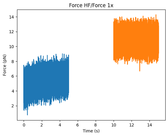
Plotting is typically performed with the origin of the plot set to the timestamp of the start of the slice. Sometimes, you may want to plot two slices together that have different starting times. You can pass a custom reference timestamp to the plotting function to make sure they use the same time shift:
first_slice = file.force1x['5s':'10s']
second_slice = file.force1x['15s':'20s']

plt.figure()
first_slice.plot()
second_slice.plot(start=first_slice.start)  # we want to use the start of first_slice as time point "zero"
plt.show()
1.2.2. Boolean array indexing
Similarly, a subset of the data can be selected using boolean array indexing. For example, forces above 5 pN can be excluded as follows:
mask = file.force1x.data <= 5
masked = file.force1x[mask]
Multiple criteria can be combined by using numpy’s logic operators.
For example, restricting the forces between 2 and 5 can be accomplished as follows:
mask = np.logical_and(file.force1x.data > 2, file.force1x.data < 5)
masked = file.force1x[mask]
1.2.3. Arithmetic
Simple arithmetic operations can be performed directly on slices:
>>> diff_force = (file.force1x - file.force2x) / 2
<lumicks.pylake.channel.Slice at 0x2954d3016d0>

>>> force_magnitude = (file.force1x**2 + file.force1y**2) ** 0.5
<lumicks.pylake.channel.Slice at 0x2954d3016d0>
1.2.4. Downsampling
A slice can be downsampled using various methods.
To downsample to a specific frequency use downsampled_to with the desired frequency in Hz:
channel = file.force1x # original frequency 78125 Hz
timestep = np.diff(channel.timestamps[:2]) * 1e-9        # timestep 12.8 us

ds_channel = channel.downsampled_to(31.25)
ds_timestep = np.diff(ds_channel.timestamps[:2]) * 1e-9  # timestep 320 us
By default, this method will take the mean of every N samples where N is defined as the ratio between the two sampling times.
This can cause issues when N isn’t an integer, leading to an unequal number of points contributing to each point in the
downsampled channel. To automatically find the nearest higher frequency that will fulfill this requirement, use the method="ceil":
ds_channel2 = channel.downsampled_to(31.26, method="ceil")
ds_timestep2 = np.diff(ds_channel2.timestamps[:2]) * 1e-9  # timestep 307.2 us
For data that is recorded with variable sampling frequencies, it is usually not possible to downsample to a
single sample rate, while maintaining an equal number of samples per downsampled sample. To force downsampling
to a single frequency in the case of variable sample rates, use method="force":
variable_channel = file.distance1
variable_ds_channel = variable_channel.downsampled_to(10, method="force")
Note that this same flag can also be used to force a specific downsampling rate for non-integer downsampling rates.
A slice can also be downsampled over arbitrary time segments by using downsampled_over and supplying a
list of (start, stop) tuples indicating over which ranges to apply the function.
A slice that contains equally spaced timestamps can be downsampled by a specific factor using downsampled_by
(note that the ratio of the original/final sampling frequencies must be an integer.):
channel = file.force1x # original frequency 78125 Hz
timestep = np.diff(channel.timestamps[:2]) * 1e-9        # timestep 12.8 us

ds_channel = channel.downsampled_by(5)
ds_timestep = np.diff(ds_channel.timestamps[:2]) * 1e-9  # timestep 64 us
Sometimes, one may want to downsample a high frequency channel in exactly the same way that a Bluelake low frequency
channel is sampled. For this purpose you can use downsampled_like:
d_data = file["Distance"]["Distance 1"]
hf_downsampled, d_cropped = file["Force HF"]["Force 1x"].downsampled_like(d_data)

plt.figure()
d_cropped.plot()
hf_downsampled.plot()
plt.show()
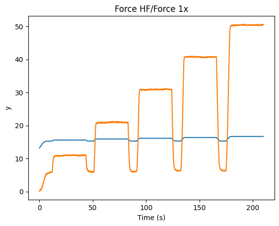
Generally, it is not possible to reconstruct the first 1-2 timepoints of the reference low frequency channel from the high frequency channel input. Therefore, this method returns the downsampled channel and a copy of the reference channel that is cropped such that both channels have exactly the same timestamps.
1.3. Calibrations
Calibration information for force channels can be found by checking the calibration member. This gives a list of calibrations:
>>> print(file.force1x.calibration)
[{'Kind': 'Discard all calibration data', 'Offset (pN)': 0.0, 'Response (pN/V)': 1.0, 'Sign': 1.0, 'Start time (ns)': 0, 'Stop time (ns)': 0}]
The actual values can be obtained from the list as follows, where the index refers to the calibration entry and the name to the actual field value:
>>> file.force1x.calibration[0]["Offset (pN)"]
0.0
If we slice a force channel, we only obtain the calibrations relevant for the selected region.
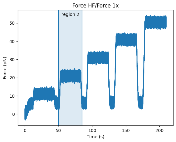
1.4. Highlighting
Let’s say something interesting happens in our data and we would like to mark a particular time region.
We can use the function highlight_time_range() for this.
We can highlight a range using the same syntax as slicing:
force = file.force1x
force.plot()
force.highlight_time_range(("50s", "85s"), annotation="region 2")
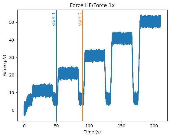
or just mark individual points:
force = file.force1x
force.plot()
force.highlight_time_range("50s", annotation="start 1", color="C0")
force.highlight_time_range("90s", annotation="start 2", color="C1")
You can even pass timeline items such as markers, but more on that in the next section.
1.5. Markers
We can see that the file also contains markers. These can be accessed from the markers attribute which returns a dictionary of markers.
>>> print(file.markers)
{'Tether: 11': <lumicks.pylake.marker.Marker object at 0x000001781E701C00>}
The actual markers can be obtained from the dictionary as follows:
>>> file.markers["Tether: 11"]
<lumicks.pylake.marker.Marker at 0x1785ccf1990>
We can find the start and stop timestamps with .start and .stop.
>>> print(file.markers["Tether: 11"].start)
1638534506519544400
>>> print(file.markers["Tether: 11"].stop)
1638534716503544401
You can slice channels directly using these timestamps:
>>> marker = file.markers["Tether: 11"]
>>> file.force1x[marker.start:marker.stop]
<lumicks.pylake.channel.Slice at 0x1785ccf1390>
You can also slice channel data directly using markers (or any other item that has a .start and .stop property):
>>> file.force1x[file.markers["Tether: 11"]]
<lumicks.pylake.channel.Slice at 0x1785ccf1390>
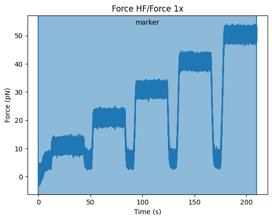
You can visualize the region of these markers superimposed on the channel data:
file.force1x.plot()
file.force1x.highlight_time_range(file.markers["Tether: 11"], annotation="marker")
1.6. Exporting h5 files
We can save the Bluelake HDF5 file to a different filename by using save_as(). When
transferring data, it can be beneficial to omit some channels from the h5 file, or use a higher compression ratio. In
particular, high frequency channels tend to take up a lot of space, and aren’t always necessary for every analysis:
file.save_as("no_hf.h5", omit_data={"Force HF/*"}) # Omit high frequency force data from export
We use fnmatch patterns for specifying which fields to omit from the saved h5 file; the * in the line of code above means that any channel starting with ""Force HF/"" should be omitted from the file.