4. Kymographs¶

Download this page as a Jupyter notebook

We can download the data needed for this tutorial directly from Zenodo using Pylake. Since we don’t want it in our working folder, we’ll put it in a folder called "test_data":

filenames = lk.download_from_doi("10.5281/zenodo.7729525", "test_data")

We can use the lk.File.kymos attribute to access the kymographs from a file:

import lumicks.pylake as lk

file = lk.File("test_data/kymo.h5")
print(file.kymos)  # dict of available kymos: {'16': Kymo(pixels=699)}

This is a regular Python dictionary so we can easily iterate over it:

# print some details for all kymos in a file
for name, kymo in file.kymos.items():
    print(f"kymograph '{name}', starts at {kymo.start} ns")

# kymograph '16', starts at 1638534513847557200 ns

Or access a particular Kymo object directly to work with:

# use the kymo name as a dict key
kymo = file.kymos["16"]

4.1. Plotting and exporting¶

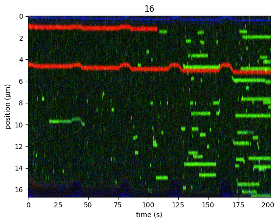
Pylake provides a convenience plot() method to quickly visualize your data. For details and examples see the Plotting Images section.

The kymograph can also be exported to TIFF format:

kymo.export_tiff("image.tiff")

4.2. Kymo data and details¶

We can access the raw image data as a numpy.ndarray:

rgb = kymo.get_image("rgb")  # matrix with `shape == (height, width, 3 colors)`
blue = kymo.get_image("blue")  # single color so `shape == (height, width)`

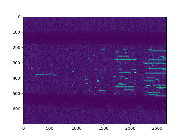
# Plot manually
plt.figure()
plt.imshow(kymo.get_image("green"), aspect="auto", vmax=15)
plt.show()

There are also several properties available for convenient access to the kymograph metadata:

kymo.center_point_um provides a dictionary of the central x, y, and z coordinates of the scan in micrometers relative to the brightfield field of view
kymo.size_um provides a list of scan sizes in micrometers along the axes of the scan
kymo.pixelsize_um provides the pixel size in micrometers
kymo.pixels_per_line provides the number of pixels in each line of the kymograph
kymo.fast_axis provides the axis that was scanned (x or y)
kymo.line_time_seconds provides the time between successive lines
kymo.pixel_time_seconds provides the pixel dwell time.
kymo.duration provides the full duration of the kymograph in seconds. This is equivalent to the number of scan lines times line_time_seconds.

4.3. Slicing, cropping & flipping¶

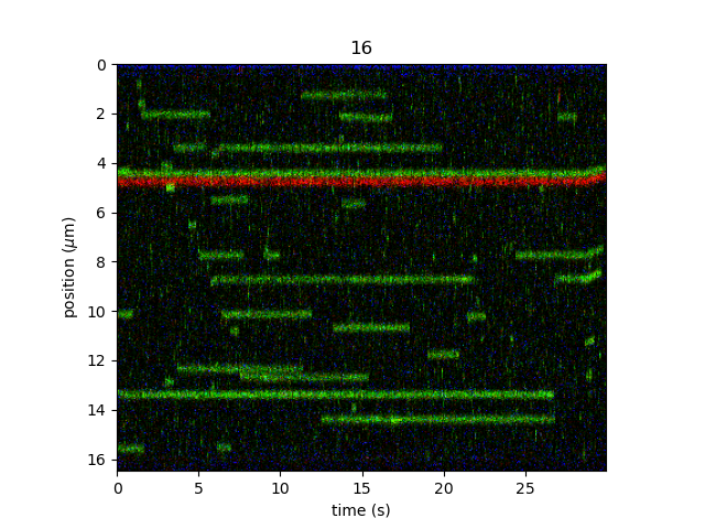
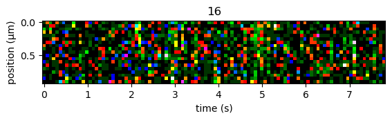
Kymographs can be sliced in order to obtain a specific time range. For example, one can plot the region of the kymograph between 130 and 160 seconds using:

plt.figure()
kymo["130s":"160s"].plot("rgb", adjustment=lk.ColorAdjustment(0, 98, mode="percentile"))
plt.show()

It is possible to crop a kymograph to a specific coordinate range, by using the function Kymo.crop_by_distance(). For example, we can crop the region from 9.5 micron to 26 microns using the following command:

plt.figure()
kymo.crop_by_distance(9.5, 26).plot("rgb", aspect="auto", adjustment=lk.ColorAdjustment(0, 98, mode="percentile"))
plt.show()

If we know the bead diameter, we can automatically crop the kymo to an estimate of the bead edges using crop_beads(). This can be convenient when batch processing many kymographs:

plt.figure()
kymo.crop_beads(4.84, algorithm="brightness").plot("rgb", aspect="auto", adjustment=lk.ColorAdjustment(0, 98, mode="percentile"))
plt.show()

Note

Note, slicing in time is currently only supported for unprocessed kymographs. If you want to both crop and slice a kymo, the order of operations is important – you need to slice before cropping:

kymo_sliced = kymo["130s":"160s"]
kymo_cropped = kymo_sliced.crop_by_distance(9.5, 26)

plt.figure()
kymo_cropped.plot("rgb", adjustment=lk.ColorAdjustment(0, 99.9, mode="percentile"))
plt.show()

If you try to slice a kymograph that has already been cropped, a NotImplementedError will be raised.

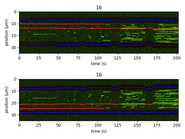
Finally, we can also flip a kymograph along its positional axis using flip(). This returns a new (but flipped) Kymo:

kymo_flipped = kymo.flip()

plt.figure()
plt.subplot(211)
kymo.plot("rgb", adjustment=lk.ColorAdjustment(0, 98, mode="percentile"))

plt.subplot(212)
kymo_flipped.plot("rgb", adjustment=lk.ColorAdjustment(0, 98, mode="percentile"))

plt.tight_layout()
plt.show()

4.4. Extracting photon counts¶

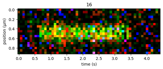
Photon counts can be extracted from the raw image, for example for stoichiometry analysis. First, select a region for which the photon counts have to be determined:

kymo_selection = kymo["88.5s":"93s"].crop_by_distance(21.4, 22.3)

plt.figure()
kymo_selection.plot("rgb", adjustment=lk.ColorAdjustment(0, 98, mode="percentile"))

Get the raw data (photon counts for each pixel) for the selected region:

selection_green = kymo_selection.get_image(channel="green")

If the background has to be subtracted, choose a region without binding events as background:

background =  kymo["92.1s":"100s"].crop_by_distance(21.4, 22.3)

plt.figure()
background.plot("rgb", adjustment=lk.ColorAdjustment(0, 98, mode="percentile"))

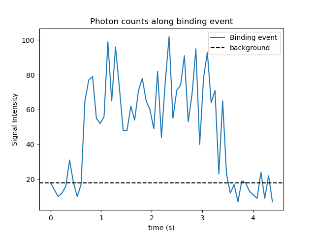
Sum over the vertical axis (along the width of the binding event) to obtain the total photon counts over the selected regions. Since every pixel has an average background signal of background_mean, we need to sum the background over the same region to obtain the total background:

summed_photon_counts = np.sum(selection_green, axis=0)
background_mean = np.mean(background.get_image(channel="green"))
summed_background = background_mean * selection_green.shape[0]
time = np.arange(len(summed_photon_counts)) * kymo.line_time_seconds

plt.figure()
plt.plot(time, summed_photon_counts, label = "Binding event")
plt.axhline(summed_background, color='k', linestyle='--', label = "background")
plt.xlabel("time (s)")
plt.ylabel("Photon counts")
plt.title("Photon counts along binding event")
plt.legend()

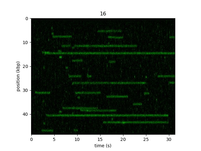
4.5. Calibrating to base pairs¶

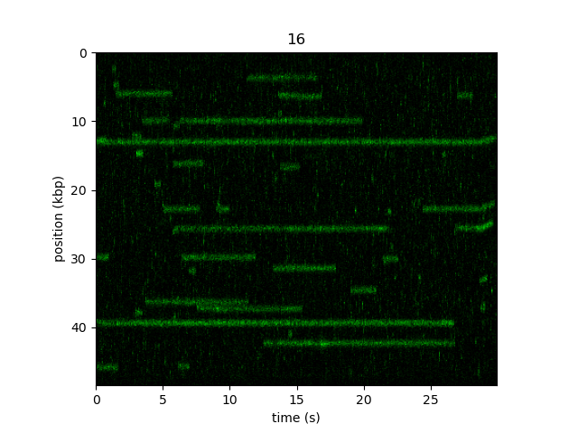
By default, kymographs are constructed with units of microns for the position axis. If, however, the kymograph spans a known length of DNA (here for example, lambda DNA) we can calibrate the position axis to kilobase pairs (kbp):

kymo_kbp = kymo_cropped.calibrate_to_kbp(48.502)

Now if we plot the image, the y-axis will be labeled in kbp:

plt.figure()
kymo_kbp.plot("green")
plt.show()

These units are also carried forward to any downstream operations such as kymotracking algorithms and MSD analysis.

Warning

Currently this is a static calibration, meaning it is only valid if the traps do not change position during the time of the kymograph.

Also, the accuracy of the calibration is dependent on how the kymo is cropped. If you crop the kymo by visually estimating the bead edges, the resulting position should be taken as approximate.

4.6. Interactive slicing, cropping & calibration¶

We can also interactively slice, crop, and calibrate kymographs using crop_and_calibrate():

widget = kymo.crop_and_calibrate(channel="rgb", tether_length_kbp=48.502, aspect="auto", adjustment=lk.ColorAdjustment(0, 99.5, mode="percentile"))

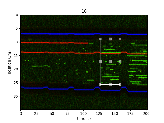
Simply click and drag the rectangle selector to the desired ROI. We can then access the edited kymograph with:

new_kymo = widget.kymo

plt.figure()
new_kymo.plot("green")
plt.show()

If the optional tether_length_kbp argument is supplied, the kymograph is automatically calibrated to the desired length in kilobase pairs. If this argument is missing (the default value None) the edited kymograph is only sliced and cropped.

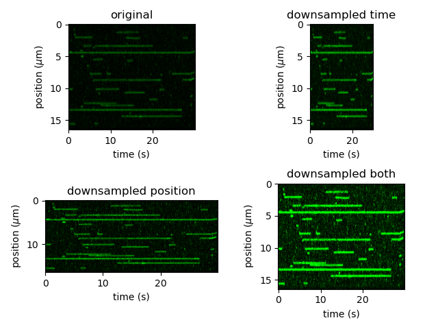
4.7. Downsampling¶

We can downsample a kymograph in time by invoking:

kymo_ds_time = kymo_cropped.downsampled_by(time_factor=2)

Or in space by invoking:

kymo_ds_position = kymo_cropped.downsampled_by(position_factor=2)

Or both:

kymo_ds = kymo_cropped.downsampled_by(time_factor=2, position_factor=2)
adjustment = lk.ColorAdjustment(0, 30, mode="absolute")

plt.figure()

plt.subplot(221)
kymo_cropped.plot("green", adjustment=adjustment)
plt.title("original")
plt.subplot(222)
kymo_ds_time.plot("green", adjustment=adjustment)
plt.title("downsampled time")
plt.subplot(223)
kymo_ds_position.plot("green", adjustment=adjustment)
plt.title("downsampled position")
plt.subplot(224)
kymo_ds.plot("green", adjustment=adjustment)
plt.title("downsampled both")

plt.tight_layout()
plt.show()

Note however, that not all functionalities are present anymore when downsampling a kymograph over time. This is because the downsampling occurs over non-contiguous sections of time (across multiple scan lines) and therefore each pixel no longer has an identifiable time. For example, we can no longer access the per pixel timestamps:

# the following line would raise a `NotImplementedError`
# kymo_ds.timestamps

Additionally, a downsampled kymograph cannot be sliced (same as cropped kymographs mentioned above). Therefore you should first slice the kymograph and then downsample.

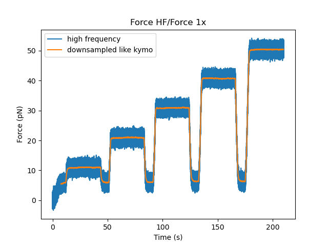
4.8. Correlating with channel data¶

We can downsample channel data according to the lines in a kymo. We can use line_timestamp_ranges() for this:

line_timestamp_ranges = kymo.line_timestamp_ranges()

This returns a list of start and stop timestamps that can be passed directly to downsampled_over(), which will then return a Slice with a datapoint per line:

force = file.force1x
downsampled = force.downsampled_over(line_timestamp_ranges)

plt.figure()
force.plot(label="high frequency")
downsampled.plot(start=force.start, label="downsampled like kymo")
plt.legend()
plt.show()

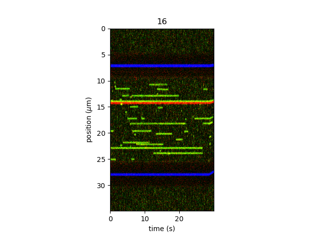
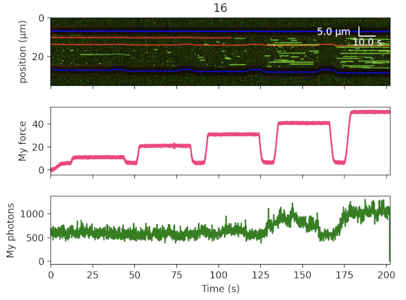
../_images/force_downsampled_like_kymo.png

We can plot a list of (multiple) channels correlated with the kymograph using plot_with_channels(). For example, we can plot the kymograph with the force downsampled by a factor 100 and the photon counts downsampled over each kymograph line as follows:

kymo.plot_with_channels(
    [
        file.force1x.downsampled_by(100),
        file["Photon count"]["Green"].downsampled_over(kymo.line_timestamp_ranges(), reduce=np.sum),
    ],
    "rgb",
    adjustment=lk.ColorAdjustment(5, 98, "percentile"),
    aspect_ratio=0.2,
    title_vertical=True,
)

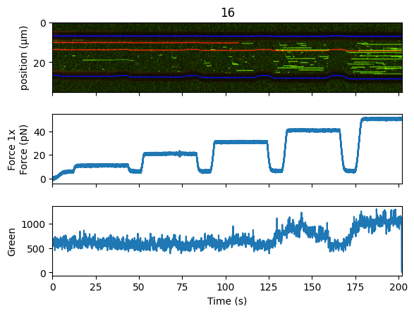
Note that in this example, we also customized the method used for downsampling the photon counts. We achieved this by passing np.sum to the reduce parameter of downsampled_over(). This results in summing the photon counts rather than taking their average. The argument title_vertical=True places the channel names along the y-axis instead of the axis title allowing a slightly more compact plot.

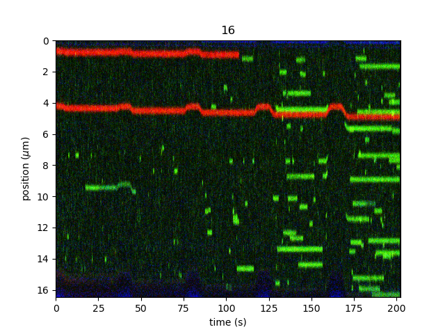
Note that the plot can be further customized by specifying custom labels, titles, colors and a scale_bar:

kymo.plot_with_channels(
    [
        file.force1x.downsampled_by(100),
        file["Photon count"]["Green"].downsampled_over(kymo.line_timestamp_ranges(), reduce=np.sum),
    ],
    "rgb",
    adjustment=lk.ColorAdjustment(5, 98, "percentile"),
    aspect_ratio=0.2,
    title_vertical=True,
    scale_bar=lk.ScaleBar(10.0, 5.0),
    colors=[[1.0, 0.2, 0.5], "green"],
    labels=["My force", "My photons"],
    titles=["", "Step-wise forces", "Line-averaged photons"],
)

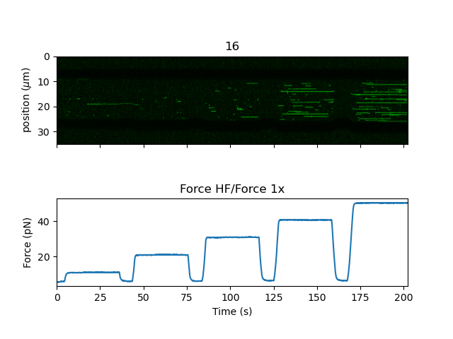
../_images/kymo_plot_with_channels_customized.png

There is also a convenience function plot_with_force() to plot a kymograph along with a downsampled force trace:

kymo.plot_with_force("1x", "green", adjustment=lk.ColorAdjustment(0, 15))

This will average the forces over each Kymograph line and plot them in a correlated fashion. The function can also take a dictionary of extra arguments to customize the kymograph plot. These parameter values get forwarded to matplotlib.pyplot.imshow().