4. RecA Fd Fitting
Download this page as a Jupyter notebook
4.1. RecA Fd Fitting
RecA is a protein that is involved in DNA repair. In this notebook, we analyze data acquired in the presence and absence of RecA. RecA forms nucleoprotein filaments on DNA and is able to mechanically modify the DNA structure. Here, we quantify these changes using the worm-like chain model.
Let’s first load our data and see which curves are present in these files:
>>> filenames = lk.download_from_doi("10.5281/zenodo.7729929", "test_data")
>>> control_file = lk.File("test_data/fdcurve.h5")
>>> reca_file = lk.File("test_data/fdcurve_reca.h5")

>>> print(control_file.fdcurves)
>>> print(reca_file.fdcurves)

{'FD_5_control_forw': <lumicks.pylake.fdcurve.FdCurve object at 0x0000022C8514E780>}
{'FD_5_3_RecA_forw_after_2_quick_manual_FD': <lumicks.pylake.fdcurve.FdCurve object at 0x0000022C8514E860>}
4.2. Plot the data
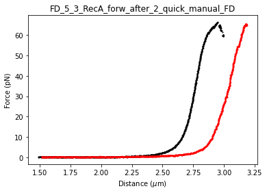
We see that each of the files has just one Fd curve. We can access the Fd curves by invoking control_file[curve_name],
or alternatively, since there’s only one, we can simply use popitem. Let’s have a quick look at the data:
control_name, control_curve = control_file.fdcurves.popitem()
reca_name, reca_curve = reca_file.fdcurves.popitem()

control_curve.plot_scatter(s=1, c="k")
reca_curve.plot_scatter(s=1, c="r")
4.3. Set up the model
For this we want to use an inverted worm-like chain model. We also include an estimated distance and force offset:
model = lk.ewlc_odijk_force("DNA").subtract_independent_offset() + lk.force_offset("DNA")
We would like to fit this model to some data. So let’s make a FdFit:
fit = lk.FdFit(model)
Let’s have a look at the parameters in this model:
>>> print(model.parameter_names)

['DNA/d_offset', 'DNA/Lp', 'DNA/Lc', 'DNA/St', 'kT', 'DNA/f_offset']
4.4. Load the data
We have to be careful when loading the data, as the Odijk worm-like chain model is only valid for intermediate forces (0 - 30 pN). That means we’ll have to crop out the section of the data that’s outside this range. We can do this by creating a logical mask which is true for the data we wish to include and false for the data we wish to exclude.
The data in an FdCurve can be referenced by invoking the f and d attribute for force and distance respectively. This
returns Slice objects, from which we can extract the data by calling .data. Since we have to do this twice, let’s
make a little function that extracts the data from the FdCurve and filters it:
def extract_data(fdcurve, f_min, f_max):
    f = fdcurve.f.data
    d = fdcurve.d.data
    mask = (f < f_max) & (f > f_min)
    return f[mask], d[mask]

force_control, distance_control = extract_data(control_curve, 0, 30)
force_reca, distance_reca = extract_data(reca_curve, 0, 30)
We can load data into the FdFit by using the function add_data:
fit.add_data("Control", force_control, distance_control)
If parameters are expected to differ between conditions, we can rename them for a specific data set when adding data to
the fit. For the second data set, we expect the contour length, persistence length and stiffness to be different, so
let’s rename these. We can do this by passing an extra argument named params. This argument takes a dictionary. The
keys of this dictionary have to be given by the original name of the parameter in the model. This name is typically
given by the name of the model followed by a slash and then the model parameter name. The value of this dictionary
should be set to the model name slash the new parameter name. Let’s rename the contour length Lc, persistence length
Lp and stretch modulus St for this data set:
fit.add_data("RecA", force_reca, distance_reca,
             params={"DNA/Lc": "DNA/Lc_RecA", "DNA/Lp": "DNA/Lp_RecA",
                     "DNA/St": "DNA/St_RecA"})
4.5. Set up the fit
Let’s add some custom parameter bounds:
fit["DNA/Lp"].value = 50
fit["DNA/Lp"].lower_bound = 39
fit["DNA/Lp"].upper_bound = 80

fit["DNA/St"].value = 1200
fit["DNA/St"].lower_bound = 700
fit["DNA/St"].upper_bound = 2000
4.6. Fit the model
Everything is set up now and we can proceed to fit the model:
>>> fit.fit()

Fit
  - Model: DNA(x-d)_with_DNA
  - Equation:
      f(d) = argmin[f](norm(DNA.Lc * (1 - (1/2)*sqrt(kT/(f*DNA.Lp)) + f/DNA.St)-(d - DNA.d_offset))) + DNA.f_offset

  - Data sets:
    - FitData(Control, N=884)
    - FitData(RecA, N=1030, Transformations: DNA/Lp → DNA/Lp_RecA, DNA/Lc → DNA/Lc_RecA, DNA/St → DNA/St_RecA)

  - Fitted parameters:
    Name                 Value  Unit      Fitted      Lower bound    Upper bound
    ------------  ------------  --------  --------  -------------  -------------
    DNA/d_offset    -0.0716458  [au]      True               -0.1            0.1
    DNA/Lp          55.7977     [nm]      True               39             80
    DNA/Lc           2.83342    [micron]  True                0            inf
    DNA/St        1407.65       [pN]      True              700           2000
    kT               4.11       [pN*nm]   False               0              8
    DNA/f_offset     0.0697629  [pN]      True               -0.1            0.1
    DNA/Lp_RecA     90.2603     [nm]      True                0            100
    DNA/Lc_RecA      3.04193    [micron]  True                0            inf
    DNA/St_RecA    846.33       [pN]      True                0            inf
4.7. Plot the fit
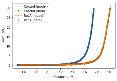
Calling the plot function on the FdFit (i.e. fit.plot()) plots the fit alongside the data:
fit.plot()
plt.ylabel("Force [pN]")
plt.xlabel("Distance [$\\mu$M]")
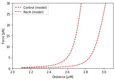
We would like to compare the two modelled curves without the data. Since we named our data sets, we can simply plot them
with their respective names. Instead this time, we specify plot_data = False to indicate that we do not wish to plot
the data this time:
fit.plot("Control", "r--", np.arange(2.1, 5.0, 0.01), plot_data=False)
fit.plot("RecA", "r--", np.arange(2.1, 5.0, 0.01), plot_data=False)
plt.ylabel("Force [pN]")
plt.xlabel("Distance [$\\mu$M]")
plt.ylim([0, 30])
plt.xlim([2, 3.1])
Let’s print the contour length difference due to RecA. We multiply by 1000 since we desire this value in nanometers:
>>> delta_lc = (fit["DNA/Lc_RecA"].value - fit["DNA/Lc"].value) * 1000.0
>>> print(f"Contour length difference: {delta_lc:.2f} [nm]")

Contour length difference: 208.51 [nm]
4.8. Try another model
There are more models in pylake. We can also try the Marko Siggia model for instance and see if it fits this data any differently:
ms_model = lk.ewlc_marko_siggia_force("DNA").subtract_independent_offset() + lk.force_offset("DNA")
ms_fit = lk.FdFit(ms_model)
ms_fit.add_data("Control", force_control, distance_control)
ms_fit.add_data("RecA", force_reca, distance_reca,
                        params={"DNA/Lc": "DNA/Lc_RecA", "DNA/Lp": "DNA/Lp_RecA",
                                "DNA/St": "DNA/St_RecA"})
ms_fit.fit();
4.9. Plot the competing models
Let’s plot the models side by side, so we can get an idea of which model fits best:
plt.figure(figsize=(20,5))
plt.subplot(1, 2, 1)
fit.plot()
plt.title("Odijk")
plt.ylim([0,10])
plt.subplot(1, 2, 2)
ms_fit.plot()
plt.title("Marko-Siggia")
plt.ylim([0,10])
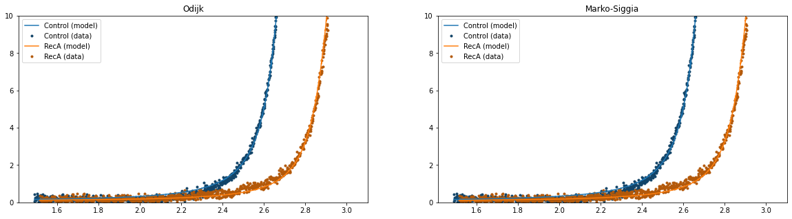
At first glance, the model fits look very similar. Since we were interested in the contour length changes, let’s have a look at what these models predict for the change in contour length:
>>> delta_lc = (fit["DNA/Lc_RecA"].value - fit["DNA/Lc"].value) * 1000.0
>>> print(f"Contour length difference Odijk: {delta_lc:.2f} [nm]")
>>> delta_lc = (ms_fit["DNA/Lc_RecA"].value - ms_fit["DNA/Lc"].value) * 1000.0
>>> print(f"Contour length difference Marko-Siggia: {delta_lc:.2f} [nm]")

Contour length difference Odijk: 208.51 [nm]
Contour length difference Marko-Siggia: 210.33 [nm]
These results are very similar, increasing our confidence in the result.
4.10. Which fit is statistically optimal
We can also determine how well a model fits the data by looking at the corrected Akaike Information Criterion and Bayesian Information Criterion. Here, a low value indicates a better model.
We can see here that both criteria seem to indicate that the Odijk model provides the best fit. Please note however, that it is always important to verify that the model produce sensible results. More freedom to fit parameters, will almost always lead to an improved fit, and this additional freedom can lead to fits that produce non-physical results. Information criteria tend to try and penalize unnecessary over-fitting, but they do not guard against unphysical parameter values.
Generally, it is always a good idea to try multiple models, and multiple sets of bound constraints, to get a feel for how reliable the estimates are:
>>> print("Corrected Akaike Information Criterion")
>>> print(f"Odijk Model with force offset {fit.aicc}")
>>> print(f"Marko-Siggia Model with force offset {ms_fit.aicc}")
>>> print("Bayesian Information Criterion")
>>> print(f"Odijk Model with force offset {fit.bic}")
>>> print(f"Marko-Siggia Model with force offset {ms_fit.bic}")

Corrected Akaike Information Criterion
Odijk Model with force offset 266.0174147701515
Marko-Siggia Model with force offset 285.1340433325082
Bayesian Information Criterion
Odijk Model with force offset 310.3974287950736
Marko-Siggia Model with force offset 329.5140573574303
We can also quickly compare parameter values:
>>> fit.params

Name                 Value  Unit      Fitted      Lower bound    Upper bound
------------  ------------  --------  --------  -------------  -------------
DNA/d_offset    -0.0716458  [au]      True               -0.1            0.1
DNA/Lp          55.7977     [nm]      True               39             80
DNA/Lc           2.83342    [micron]  True                0            inf
DNA/St        1407.65       [pN]      True              700           2000
kT               4.11       [pN*nm]   False               0              8
DNA/f_offset     0.0697629  [pN]      True               -0.1            0.1
DNA/Lp_RecA     90.2603     [nm]      True                0            100
DNA/Lc_RecA      3.04193    [micron]  True                0            inf
DNA/St_RecA    846.33       [pN]      True                0            inf

>>> ms_fit.params

Name                 Value  Unit      Fitted      Lower bound    Upper bound
------------  ------------  --------  --------  -------------  -------------
DNA/d_offset    -0.1        [au]      True               -0.1            0.1
DNA/Lp          58.377      [nm]      True                0            100
DNA/Lc           2.86002    [micron]  True                0            inf
DNA/St        1400.35       [pN]      True                0            inf
kT               4.11       [pN*nm]   False               0              8
DNA/f_offset     0.0468744  [pN]      True               -0.1            0.1
DNA/Lp_RecA     91.857      [nm]      True                0            100
DNA/Lc_RecA      3.07035    [micron]  True                0            inf
DNA/St_RecA    855.266      [pN]      True                0            inf
4.11. Dynamic experiments
We can see some differences in the estimates but nothing that would be a cause for immediate concern, so let’s stick with the Odijk model for the rest of this analysis as it fits slightly better. One thing we noticed when acquiring the data was that some of the experiments showed some dynamics. It would be interesting to look at the contour length changes for these experiments. To this end, we take the model we just fitted and determine a contour length per data point of this model while keeping all other parameters the same.
Let’s load the data and have a look:
dynamic_file = lk.File("test_data/fd_multiple_Lc.h5")
dynamic_name, dynamic_curve = dynamic_file.fdcurves.popitem()
dynamic_curve.plot_scatter()
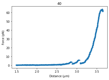
Once again, we extract our data up to 25 pN. We can reuse the function we defined earlier:
force_dynamic, distance_dynamic = extract_data(dynamic_curve, 0, 25)
4.12. A contour length per point
Now comes the more challenging part. Inverting the model for contour length. Luckily, this procedure has already been
implemented in Pylake. The function parameter_trace() inverts the model for a particular model parameter. Let’s have
a look at the parameters it needs. We can look this up in the documentation for parameter_trace()
or invoke help:
help(lk.parameter_trace)
Let’s see if we have all these pieces of information. We stored the model in the variable model. We can extract
the parameters for the RecA condition using the name we provided to the dataset before (i.e. fit["RecA"]).
The parameter we wish to invert for is DNA/Lc and for the independent and dependent variables we simply
pass the dataset:
Lcs = lk.parameter_trace(model, fit["RecA"], "DNA/Lc", distance_dynamic, force_dynamic)
Let’s plot it:
plt.plot(Lcs)
plt.ylabel("Contour lengths")
plt.xlabel("Time [s]")
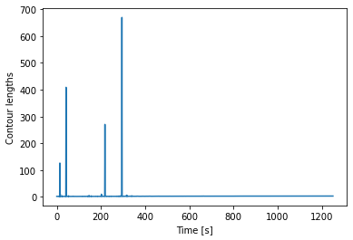
Looks like some of the estimates are way off early in the curve. Doing this inversion at very low distances is quite error prone, likely due to the non-linearity of the model. In addition, the Odijk model is known to not be reliable at low forces, so we would like to exclude this data anyway. Let’s only look at the points where the distance is higher than 2.25 micrometers:
distance_mask = distance_dynamic > 2.2

plt.plot(distance_dynamic[distance_mask], Lcs[distance_mask])
plt.ylabel("Contour length [micron]")
plt.xlabel("Distance [micron]")
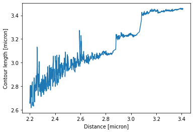
Here we can see the different contour length transitions quite clearly. There seems to be one region of contour lengths around 3.2 before finally lengthening to 3.4 micrometers.