2.1. Kymograph and Force
Download this page as a Jupyter notebook
In this experiment, two beads are trapped with a DNA attached to both of them at either end. We validated that we have a single tether of DNA by pulling on them prior to making the kymograph.
We then moved into the channel that contains Sytox-Green. It binds to DNA when the DNA is under tension. We can the scan along the DNA and create kymographs using the confocal part of the system.
By changing the force on the DNA, we can observe the force dependent binding of Sytox to DNA. This experiment perfectly demonstrates the correlative capabilities of the C-trap.
Download the files with download_from_doi():
lk.download_from_doi("10.5281/zenodo.12666983", "data")
Open the File:
file = lk.File("data/sytox_kymo.h5")
2.1.1. Read the kymographs
List all the kymographs in the File:
>>> list(file.kymos)
['7']
Load the kymograph in the File:
# You can either select the kymograph directly:
kymo_data = file.kymos["7"]  # as this file contains kymograph #7

# or alternatively you can create a list of kymograph names and simply take the first one,
# in which case you don't have to worry about which file you open:
kymo_names = list(file.kymos)
kymo = file.kymos[kymo_names[0]]
Plot the green channel:
plt.figure(figsize=(15, 10))
kymo.plot("green")
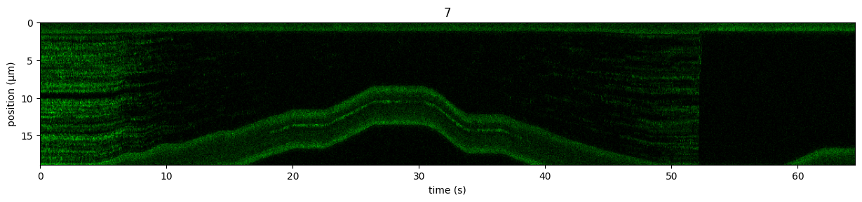
Note that we can also scale the colorbar of the image.
Get the raw data out of the Kymo:
green_data = kymo.get_image("green")
Get a sense of the pixel values in the kymos
>>> max_px = np.max(green_data)
35
>>> min_px = np.min(green_data)
0
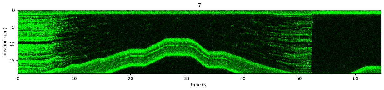
Scale the colorbar and make the Kymo look better:
plt.figure(figsize=(15,10))
kymo.plot("green", vmax=10);
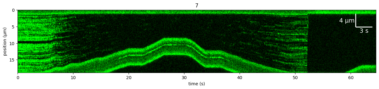
Alternatively, we can plot the kymograph using percentiles, which usually works pretty robustly without having to know the exact photon count values.
This can be achieved using a ColorAdjustment.
We can also add a ScaleBar:
plt.figure(figsize=(15,10))
scale_bar = lk.ScaleBar(3, 4, fontsize=14, barwidth=2)  # Parameters are x-axis (time) and y-axis (position)
adjustment = lk.ColorAdjustment(5, 95, "percentile")
kymo.plot("green", adjustment=adjustment, scale_bar=scale_bar);
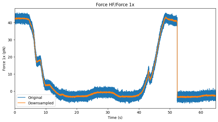
2.1.2. Force versus Time
Load the data:
# Force in the x direction (pN)
force1x = file["Force HF"]["Force 1x"]
Downsample the data using downsampled_by():
sample_rate = force1x.sample_rate
downsampled_rate = 100  # Hz
downsampling_factor = int(sample_rate / downsampled_rate)

# downsample the force, nanostage position and time
force1x_downsamp = force1x.downsampled_by(downsampling_factor)
Next, let’s plot() the force:
plt.figure(figsize=(10, 5))

force1x.plot(label="Original")
force1x_downsamp.plot(label="Downsampled")
plt.ylabel("Force 1x (pN)")
plt.xlim([0, max(force1x.seconds)])
plt.legend(loc="lower left");
2.1.3. Correlated Force and Confocal
Plot the final figure:
plt.figure(figsize=(15, 10))
plt.subplot(2, 1, 1)
kymo.plot("green", vmax=10)

plt.subplot(2, 1, 2)
force1x.plot(label="Original")
force1x_downsamp.plot(label="Downsampled")
plt.xlim([0, max(force1x.seconds)])
plt.ylabel("Force 1x (pN)");
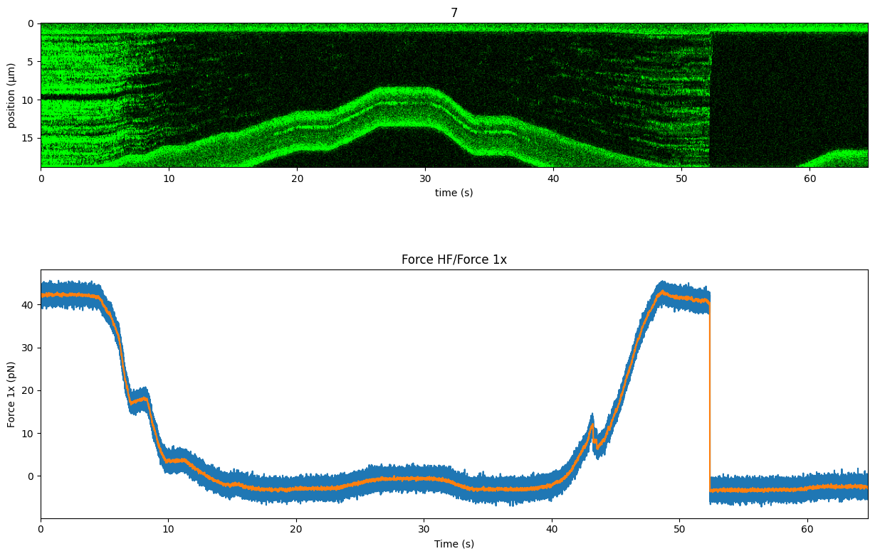
We see when we decreased the force on the DNA Sytox unbinds. As soon as we increase the tension again, Sytox starts binding again. At around 52 seconds, the DNA tether broke, which is why the force went back to it’s original value.