8. Active calibration for two beads
Download this page as a Jupyter notebook
When performing active calibration, the nanostage (whose motion is calibrated in microns) is oscillated sinusoidally. In turn, this results in fluid motion, which displaces the beads from the trap centers. We can detect this sinusoidal displacement on the force detectors and use it to calibrate the displacement sensitivity. For the theory on how this works, please refer to the theory section on active calibration.
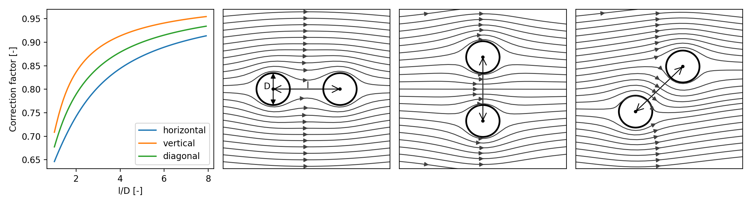
When using two beads, the flow field around the beads is reduced (because the presence of the additional bead slows down the fluid). The magnitude of this effect depends on the bead diameter, distance between the beads and their orientation with respect to the fluid flow. Streamlines for some bead configurations are shown below (simulated using FEniCSx [Dev23]).
In this notebook, we will show this effect on some C-Trap data and apply a correction for it.
Note
In practice, correcting data for this effect is straightforward and most of this notebook is not required. Considering the correction factor is a single factor that only depends on the bead to bead distance and bead radius, it can be applied as a correction factor to already calibrated data. See tutorial for more information on how to correct an experiment.
8.1. Loading the data
First, we need to download the necessary data. Note that this cell downloads 7.4 GB of data (it may take a while):
lk.download_from_doi("10.5281/zenodo.11105579", "coupling_data")
We can get a list of filenames for the files we need for each experiment using glob.glob():
import glob
from tqdm.auto import tqdm

# Grab calibration data for different beads
calibration_data = [glob.glob(f"coupling_data/bead{bead}_*.h5") for bead in ("1", "2", "3", "4", "4b", "4c")]
To perform active calibration for two beads, we will need the following:
Nanostage signals
The uncalibrated force signal in volts
Bead positions (if there is more than one bead).
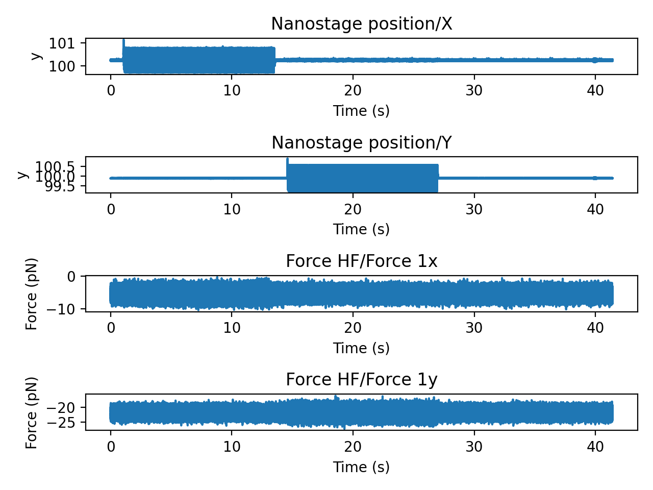
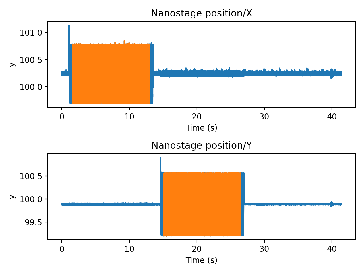
Let’s plot a typical active calibration dataset:
dataset = lk.File(calibration_data[0][0])

plt.figure()
plt.subplot(4, 1, 1)
dataset["Nanostage position"]["X"].plot()
plt.subplot(4, 1, 2)
dataset["Nanostage position"]["Y"].plot()
plt.subplot(4, 1, 3)
dataset.force1x.plot()
plt.subplot(4, 1, 4)
dataset.force1y.plot()
plt.tight_layout()
Let’s write a function that grabs the timestamp range of each oscillatory segment. Since the nanostage position shows a transient settling behavior when starting and stopping its motion, we trim a little extra time at the edges:
def find_oscillation_timestamp_range(slc, thresh=0.1, offset=0.5):
    """Search for oscillation timestamp range by thresholding signal power.

    Note: This function assumes that there is only one oscillation period in the slice.

    Parameters
    ----------
    slc : Slice
        Slice of channel data
    thresh : float
        Threshold
    offset : float
        How many seconds to trim at each edge.

    Returns
    -------
    Tuple(int64, int64)
        Returns a tuple of integer timestamps in nanoseconds.
    """

    # Calculate a downsampled mean signal power.
    zero_mean = slc - np.mean(slc.data)
    squared = (zero_mean * zero_mean).downsampled_by(100)
    start_idx = np.where(squared.data > thresh)[0][0]
    stop_idx = len(squared.data) - np.where(np.flip(squared.data) > thresh)[0][0]
    start, stop = (squared.timestamps[idx] for idx in (start_idx, stop_idx))

    # How much data do we cut at the edges? Convert the time in seconds to nanoseconds.
    trim_nanoseconds = int(offset * 1e9)

    return start + trim_nanoseconds, stop - trim_nanoseconds
Let’s plot some results and see if it identifies the regions correctly:
plt.figure()
plt.subplot(2, 1, 1)
dataset["Nanostage position"]["X"].plot()
plt.subplot(2, 1, 2)
dataset["Nanostage position"]["Y"].plot()
plt.subplot(2, 1, 1)
x_start, x_stop = find_oscillation_timestamp_range(dataset["Nanostage position"]["X"])
nano_x = dataset["Nanostage position"]["X"][x_start:x_stop]
nano_x.plot(start=dataset["Nanostage position"]["X"].start)
plt.subplot(2, 1, 2)
y_start, y_stop = find_oscillation_timestamp_range(dataset["Nanostage position"]["Y"])
nano_y = dataset["Nanostage position"]["Y"][y_start:y_stop]
nano_y.plot(start=dataset["Nanostage position"]["Y"].start)
plt.tight_layout()
To do active calibration correctly, we will need a slice containing only those chunks of data where the nanostage is oscillating. We need to de-calibrate the force (since we intend to do the calibration ourselves). And finally, we need the bead-to-bead distances. We can make a little helper function to extract these:
def read_calibration_data(h5_file, driving_axis):
"""Read active calibration data for a single axis
h5_file : lumicks.pylake.File
Opened h5 file with a single active calibration.
driving_axis : str
Which driving axis to extract data for ("x" or "y")
"""
# Grab our driving data
driving_channel = h5_file["Nanostage position"][driving_axis.upper()]
start, stop = find_oscillation_timestamp_range(driving_channel)
# Slice the data we need (data during the oscillation phase)
driving_data = driving_channel[start:stop]
volt_slices = {}
for trap in ("1", "2"):
force_data = getattr(h5_file, f"force{trap}{driving_axis}")
force_data = force_data[start:stop]
# To recalibrate, we need the signal in volts. If the force was calibrated prior to
# acquisition, we need to de-calibrate it first. We use `get` on the calibration
# dictionary here so that we can revert to a default of `1`, if the last calibration
# does not have a force sensitivity (meaning the signal was already in volts).
force_calibration = force_data.calibration[0].get("Rf (pN/V)", 1)
# We can divide directly on the slice.
volt_slices[f"{trap}{driving_axis}"] = force_data / force_calibration
# Grab the average bead positions
b1x = np.mean(h5_file["Bead position"]["Bead 1 X"][start:stop].data)
b2x = np.mean(h5_file["Bead position"]["Bead 2 X"][start:stop].data)
b1y = np.mean(h5_file["Bead position"]["Bead 1 Y"][start:stop].data)
b2y = np.mean(h5_file["Bead position"]["Bead 2 Y"][start:stop].data)
return b2x - b1x, b2y - b1y, driving_data, volt_slices
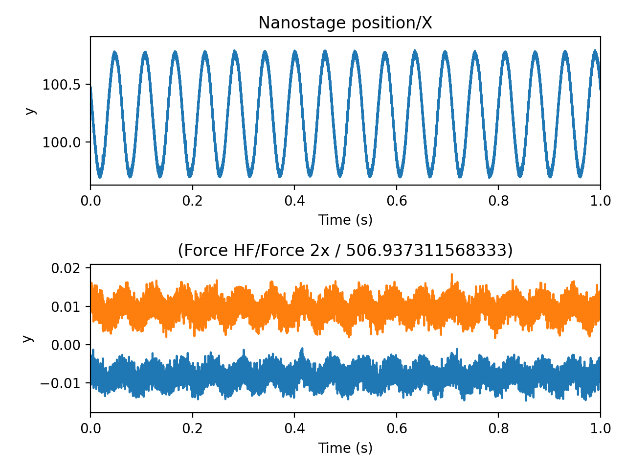
# Test our experiment reading function by looking at the first second of data
dx, dy, stage, volts = read_calibration_data(dataset, driving_axis="x")
plt.figure()
plt.subplot(2, 1, 1)
stage.plot()
plt.xlim([0, 1])
plt.subplot(2, 1, 2)
volts["1x"].plot()
volts["2x"].plot()
plt.xlim([0, 1])
plt.tight_layout()
8.2. Performing the calibrations
We define a calibration helper function to make our code more succinct:
def calibrate(psd, nano=None, *, bead_diameter, temperature, excluded_ranges):
    """Perform passive or active calibration

    Parameters
    ----------
    psd : Slice
        Slice of raw voltage data from the force detector
    nano : Slice, optional
        Slice of nanostage data. When omitted, passive calibration is performed.
    bead_diameter : float
        Bead diameter in microns
    temperature : float
        Calibration temperature
    excluded_ranges : list
        List of exclusion ranges
    """
    return lk.calibrate_force(
        force_voltage_data=psd.data,
        sample_rate=psd.sample_rate,
        bead_diameter=bead_diameter,
        temperature=temperature,
        driving_data=nano.data if nano else None,
        driving_frequency_guess=17,  # This is the default driving frequency in Bluelake
        num_points_per_block=350,
        hydrodynamically_correct=True,  # The hydrodynamically correct provides more accurate calibration
        active_calibration=True if nano else False,
        excluded_ranges=excluded_ranges,
    )
Most systems have a few exclusion ranges defined to reject narrow noise peaks.
These are system-specific ranges that are not used in the fitting procedure when calibrating.
You can find these in any calibration item obtained from Bluelake (listed as Exclusion range ## (min.) (Hz) and Exclusion range ## (max.) (Hz) for each range).
For this system, we’ll define them here:
excluded_ranges = {
    "1x": [[12, 22], [205, 265]],
    "1y": [[12, 22]],
    "2x": [[12, 22], [205, 265]],
    "2y": [[12, 22], [19505, 19565]],
}
Let’s do a passive and active calibration now.
We can plot the thermal part of the fit by calling .plot() on the calibration result:
dx, dy, stage, volts = read_calibration_data(dataset, driving_axis="x")
passive = calibrate(
    volts["1x"], bead_diameter=2.1, temperature=26.6, excluded_ranges=excluded_ranges["1x"]
)
active = calibrate(
    volts["1x"], stage, bead_diameter=2.1, temperature=26.6, excluded_ranges=excluded_ranges["1x"]
)

passive.plot()
active.plot()
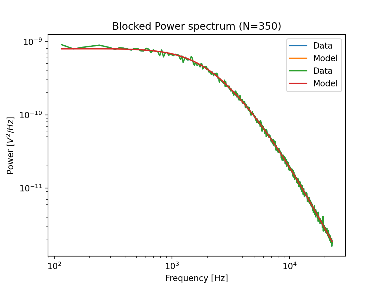
Note that the spectral fit is exactly the same for passive and active calibration. In active calibration, the peak resulting from the sinusoidal stage motion is used to directly calibrate the displacement sensitivity. As a result, active calibration does not rely on an estimate of the diffusion constant to perform the displacement sensitivity calibration, thereby reducing its reliance on assumed parameters such as viscosity, bead radius and temperature.
We can see this by changing the temperature in our calibration procedure. The result for passive calibration changes a lot, while the result for active calibration changes very little. The reason for this is that active calibration does not rely on the viscosity estimate as much (which depends strongly on temperature):
# Put some of the parameters that will be the same in a dictionary so we don't have to repeat them.
shared_pars = {"bead_diameter": 2.1, "excluded_ranges": excluded_ranges["1x"]}

print("Passive")
print(calibrate(volts["1x"], temperature=25, **shared_pars)["kappa"])
print(calibrate(volts["1x"], temperature=30, **shared_pars)["kappa"])
print("Active")
print(calibrate(volts["1x"], stage, temperature=25, **shared_pars)["kappa"])
print(calibrate(volts["1x"], stage, temperature=30, **shared_pars)["kappa"])
8.3. Analyzing the coupling dataset
Next, we define a function that calibrates all axes with both passive and active calibration for a dataset:
def calculate_calibrations(h5_file, bead_diameter, temperature):
    passive = {}
    active = {}

    for axis in ("x", "y"):
        dx, dy, stage, volts = read_calibration_data(h5_file, driving_axis=axis)
        for trap in ("1", "2"):
            shared_parameters = {
                "bead_diameter": bead_diameter,
                "temperature": temperature,
                "excluded_ranges": excluded_ranges[f"{trap}{axis}"],
            }

            passive[f"{trap}{axis}"] = calibrate(
                volts[f"{trap}{axis}"],
                **shared_parameters,  # This unpacks the dictionary into keyword arguments
            )

            active[f"{trap}{axis}"] = calibrate(
                volts[f"{trap}{axis}"],
                stage,
                **shared_parameters,  # This unpacks the dictionary into keyword arguments
            )

    return {"dx": dx, "dy": dy, "passive": passive, "active": active}
calculate_calibrations now returns the distances between the beads and all the calibration factors obtained with passive and active calibration.
>>> single_distance_result = calculate_calibrations(lk.File(calibration_data[0][0]), bead_diameter=2.1, temperature=25)
... single_distance_result["passive"]["1x"]
Let’s calculate calibration factors for all the data in this dataset.
Note that this cell may take a while to execute as it is performing 240 calibrations:
# Determine the force calibration factors for all the bead pairs in the dataset.
experiment = []
for bead_pair_files in calibration_data:
    # Determine results for a single bead pair
    bead_pair_results = []
    for calibration_file in tqdm(bead_pair_files):  # tqdm shows a progress bar
        file = lk.File(calibration_file)
        calibration = calculate_calibrations(file, bead_diameter=2.1, temperature=26.6)
        bead_pair_results.append(calibration)

    experiment.append(bead_pair_results)
Now that we have those results, let’s define some functions to conveniently extract the calibration parameters:
def extract_parameter(calibrations, calibration_type, axis, parameter):
    """Extract particular parameter for a particular experiment

    Parameters
    ----------
    calibrations : dict
        Dictionary of calibration results
    calibration_type : "active" or "passive"
        Calibration type
    axis : str
        Calibration axis (e.g. "1x")
    parameter : str
        Which parameter to extract (e.g. "kappa")
    """
    values = [cal[calibration_type][axis][parameter].value for cal in calibrations]
    return np.array(values)


def extract_distances(calibrations):
    """Extract bead distances"""
    return (np.array(s) for s in zip(*[(cal["dx"], cal["dy"]) for cal in calibrations]))
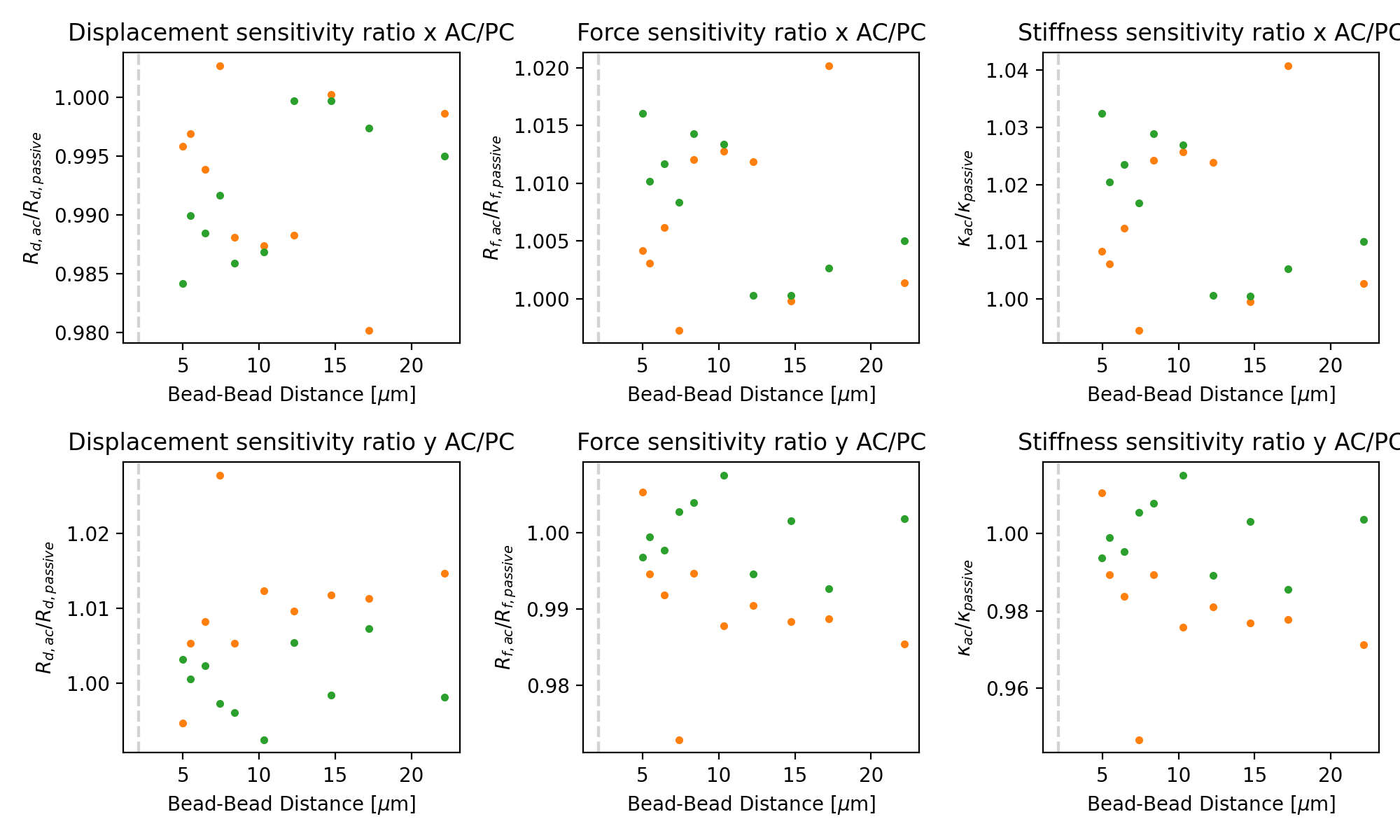
We can now show the effect of coupling on active calibration in practice using the analyzed data:
parameters = {
    "Rd": r"Displacement sensitivity [$\mu$m/V]",
    "Rf": "Force sensitivity [pN/V]",
    "kappa": "Stiffness [pN/nm]",
}

plt.figure(figsize=(10, 3))
for ix, (param, param_description) in enumerate(parameters.items()):
    plt.subplot(1, 3, ix + 1)
    dx, dy = extract_distances(experiment[0])
    plt.plot(dx, extract_parameter(experiment[0], "active", "2x", param), ".", label="active")
    plt.plot(dx, extract_parameter(experiment[0], "passive", "2x", param), "x", label="passive")
    plt.xlabel(r"Bead-Bead Distance [$\mu$m]")
    plt.ylabel(param_description)

plt.tight_layout()
plt.legend()
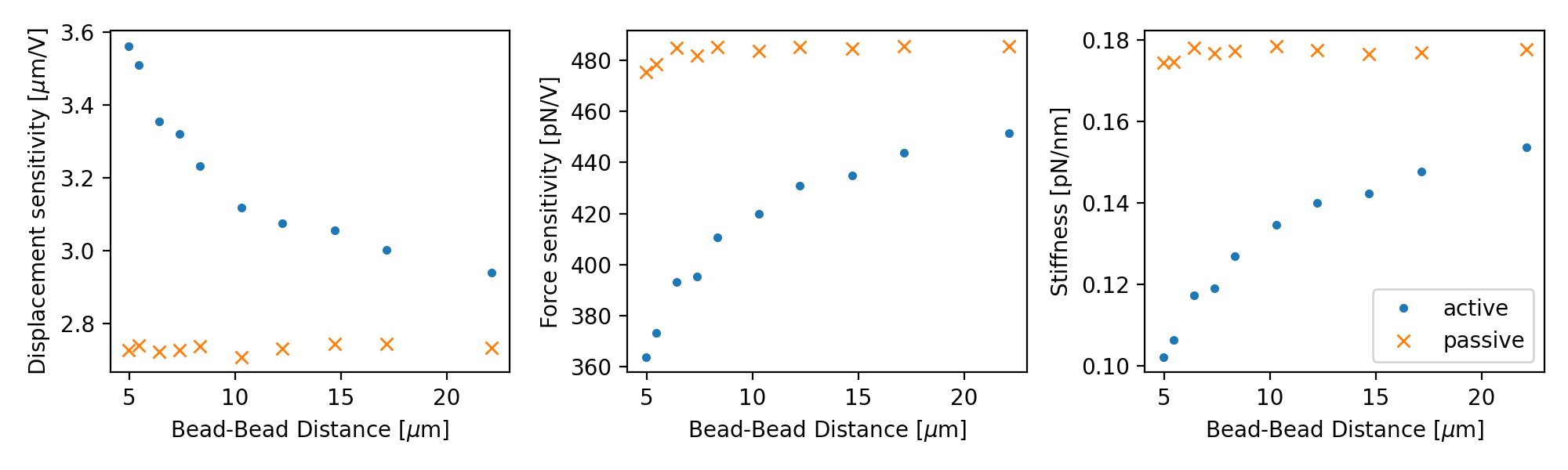
Note how the active calibration result strongly depends on the distance between the bead centers.
This is due to the reduced flow due to the presence of a second bead.
Pylake contains a model that calculates a correction factor that can be used to correct for this.
The correction factor can be obtained using coupling_correction_2d() and applied as follows:
For more information on this, please refer to the theory or tutorial. To show how well this model fits the data, we can plot it alongside the ratio of active to passive calibration:
for exp in experiment:
    plt.figure(figsize=(10, 6))
    dx, dy = extract_distances(exp)

    for trap in (1, 2):
        for ix, axis in enumerate(("x", "y")):
            plt.subplot(2, 3, 1 + 3 * ix)

            # Note that y-oscillations have a different coupling correction than x-oscillations!
            bead_diameter = 2.1
            dx_c = np.arange(3, 25, 0.1)
            c = lk.coupling_correction_2d(
                dx_c,
                np.zeros(dx_c.shape),
                bead_diameter=bead_diameter,
                is_y_oscillation=True if axis == "y" else False,
            )

            ac = extract_parameter(exp, "active", f"{trap}{axis}", "Rd")
            pc = extract_parameter(exp, "passive", f"{trap}{axis}", "Rd")
            plt.plot(dx, ac / pc, f"C{trap}.")
            plt.plot(dx_c, 1 / c, "k--")
            plt.axvline(bead_diameter, color="lightgray", linestyle="--")
            plt.xlabel(r"Bead-Bead Distance [$\mu$m]")
            plt.ylabel("$R_{d, ac} / R_{d, passive}$")
            plt.title(f"Displacement sensitivity ratio {axis} AC/PC")

            plt.subplot(2, 3, 2 + 3 * ix)
            ac = extract_parameter(exp, "active", f"{trap}{axis}", "Rf")
            pc = extract_parameter(exp, "passive", f"{trap}{axis}", "Rf")
            plt.plot(dx, ac / pc, f"C{trap}.")
            plt.plot(dx_c, c, "k--")
            plt.axvline(bead_diameter, color="lightgray", linestyle="--")
            plt.xlabel(r"Bead-Bead Distance [$\mu$m]")
            plt.ylabel("$R_{f, ac} / R_{f, passive}$")
            plt.title(f"Force sensitivity ratio {axis} AC/PC")

            plt.subplot(2, 3, 3 + 3 * ix)
            ac = extract_parameter(exp, "active", f"{trap}{axis}", "kappa")
            pc = extract_parameter(exp, "passive", f"{trap}{axis}", "kappa")
            plt.plot(dx, ac / pc, f"C{trap}.", label=f"{trap}{axis}")
            plt.plot(dx_c, c**2, "k--")
            plt.axvline(bead_diameter, color="lightgray", linestyle="--")
            plt.xlabel(r"Bead-Bead Distance [$\mu$m]")
            plt.ylabel(r"$\kappa_{ac} / \kappa_{passive}$")
            plt.title(f"Stiffness sensitivity ratio {axis} AC/PC")

            plt.tight_layout()
            plt.legend()
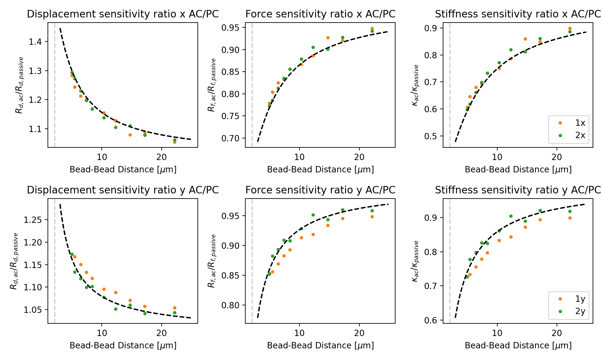
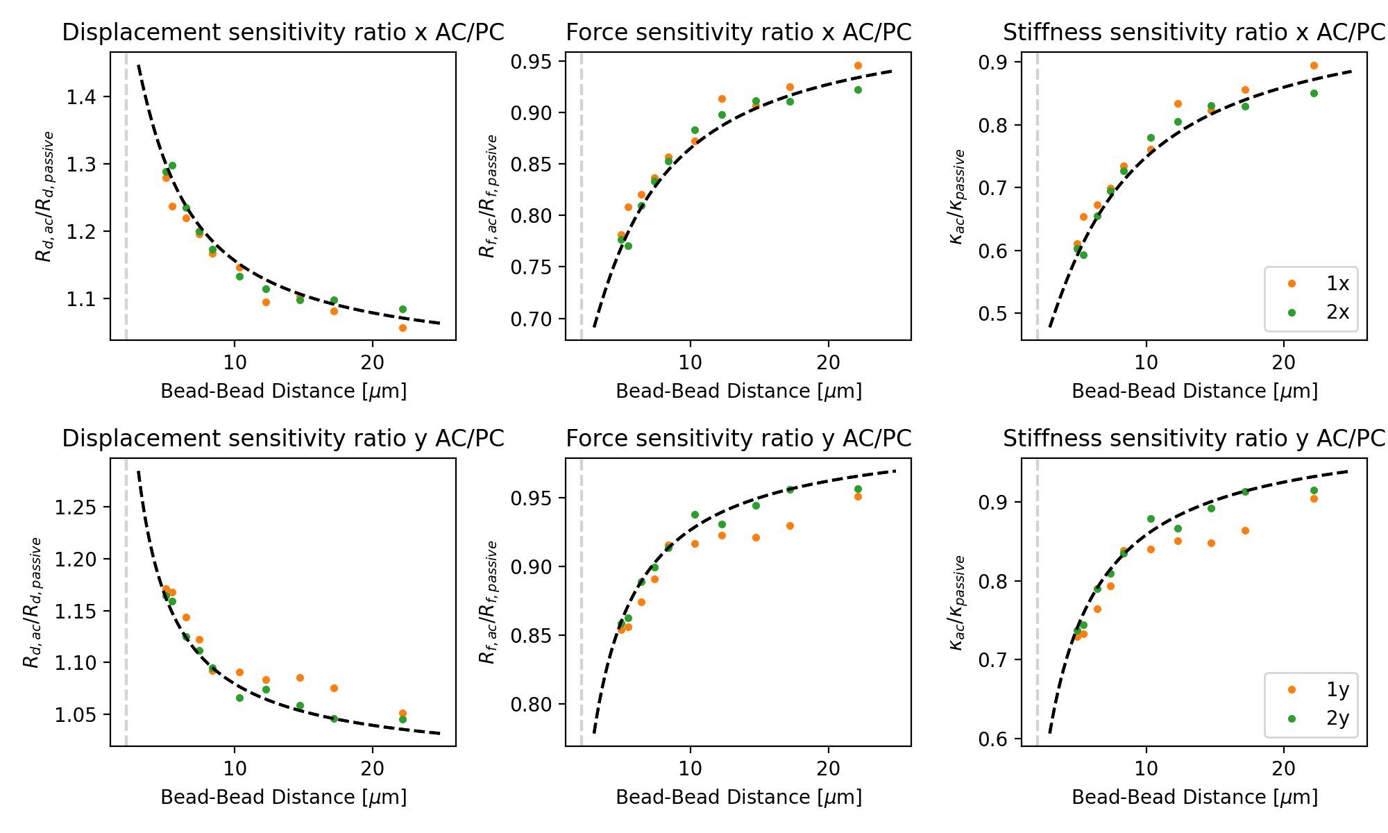
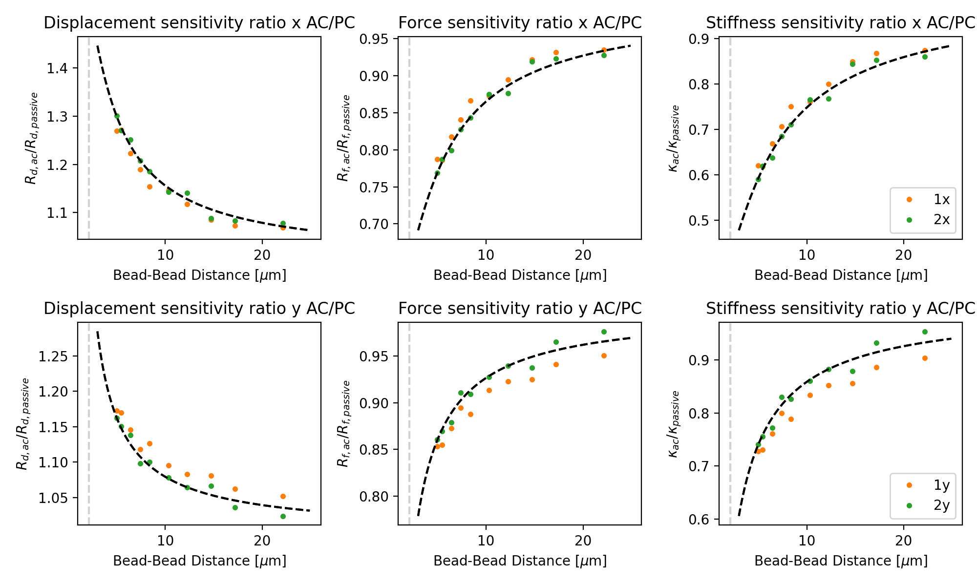
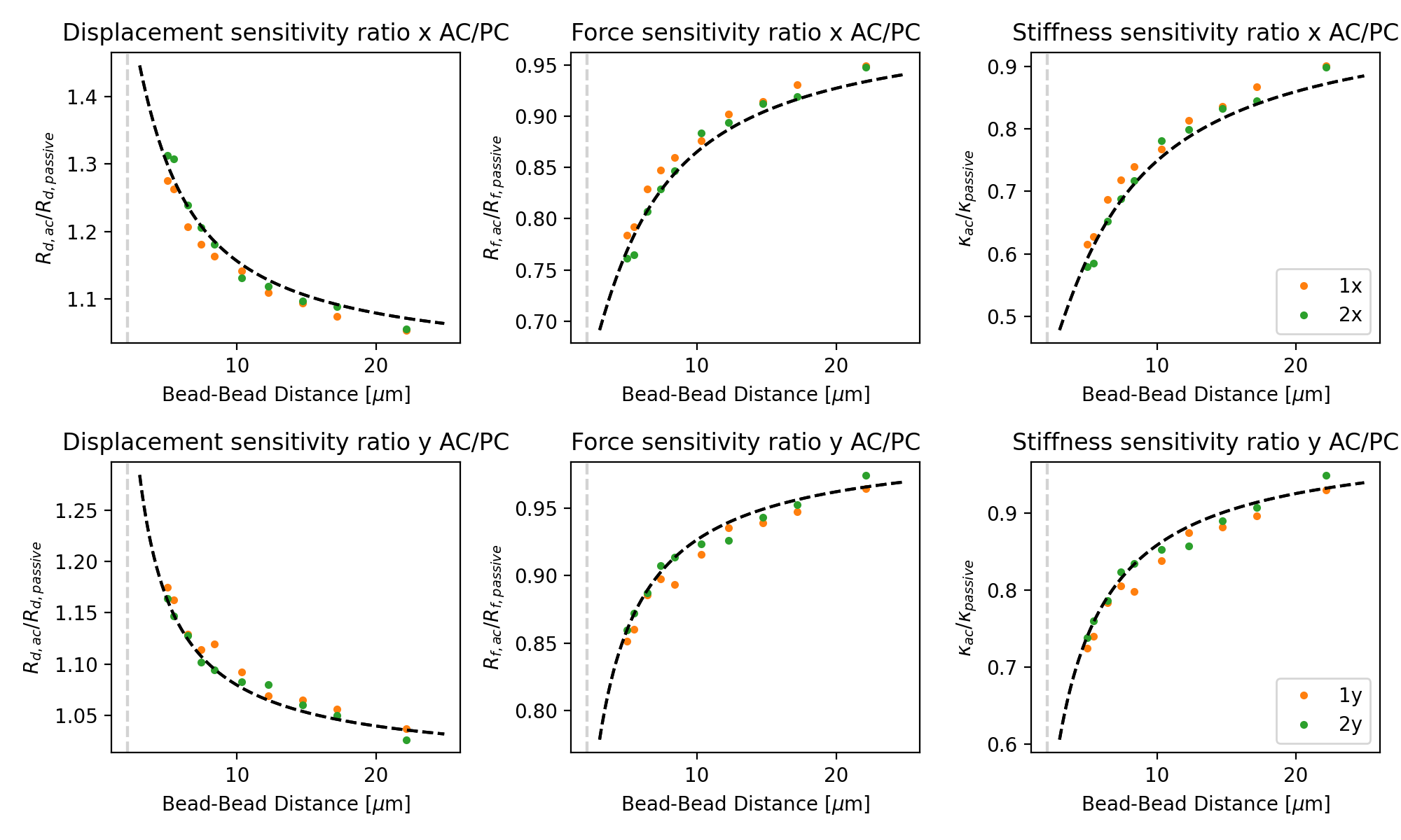
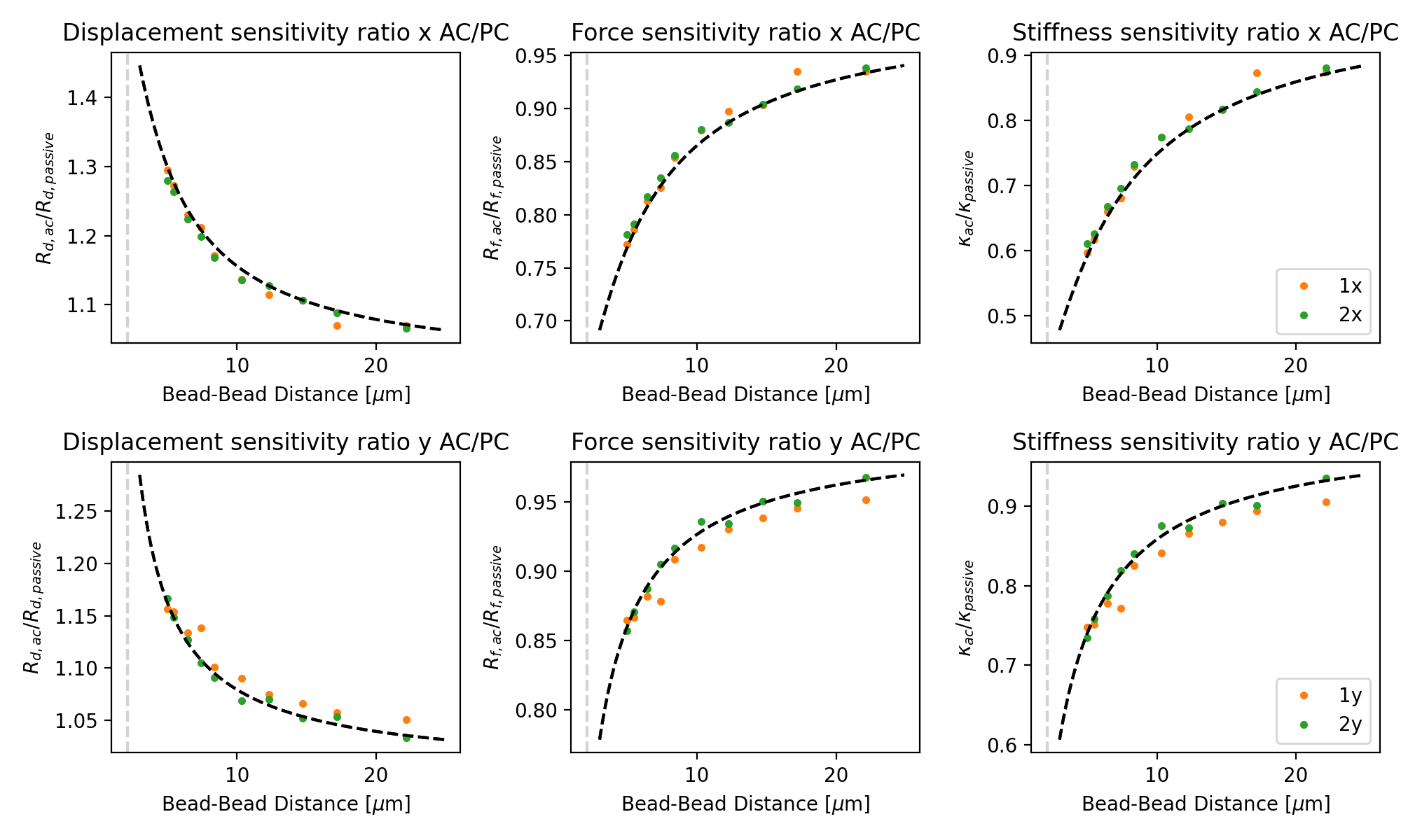
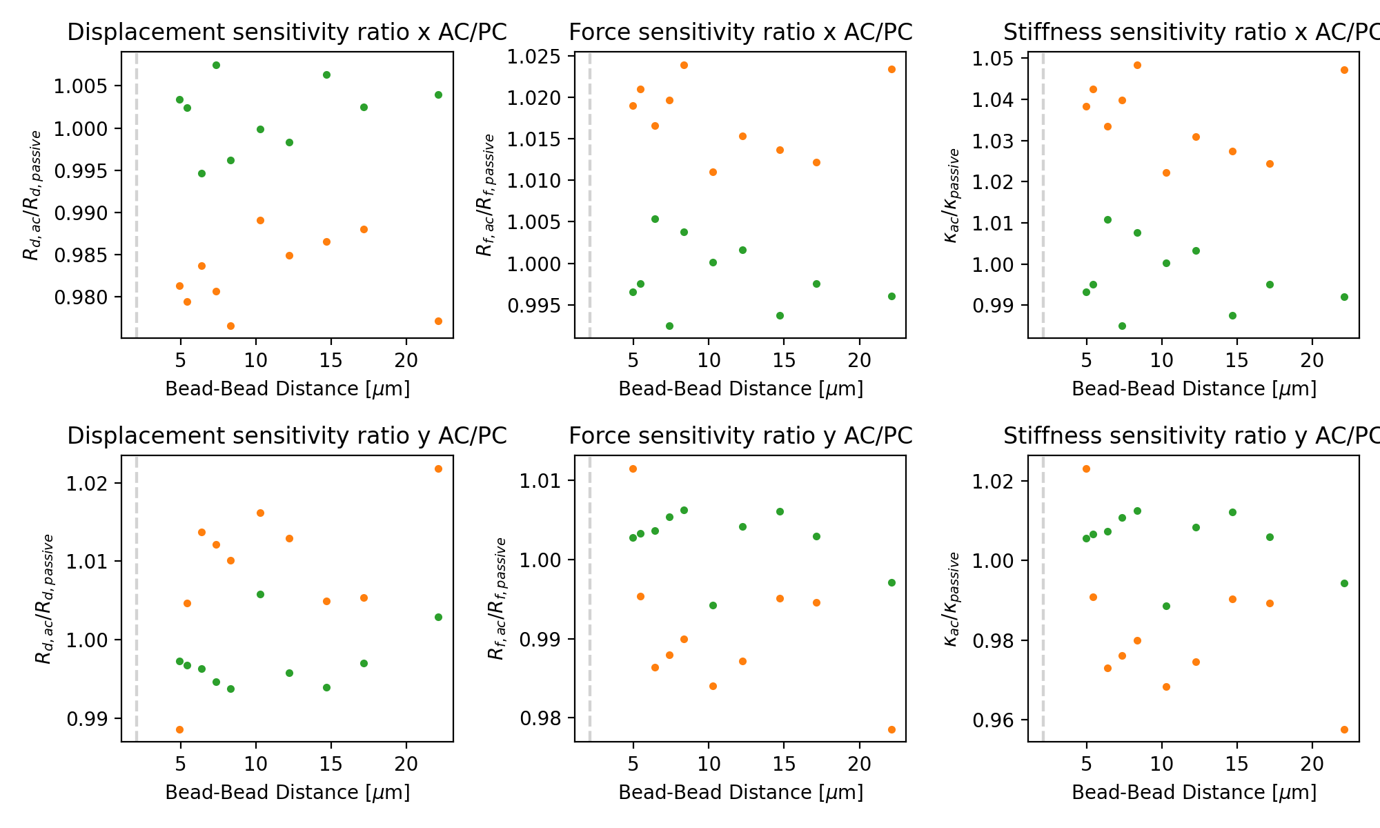
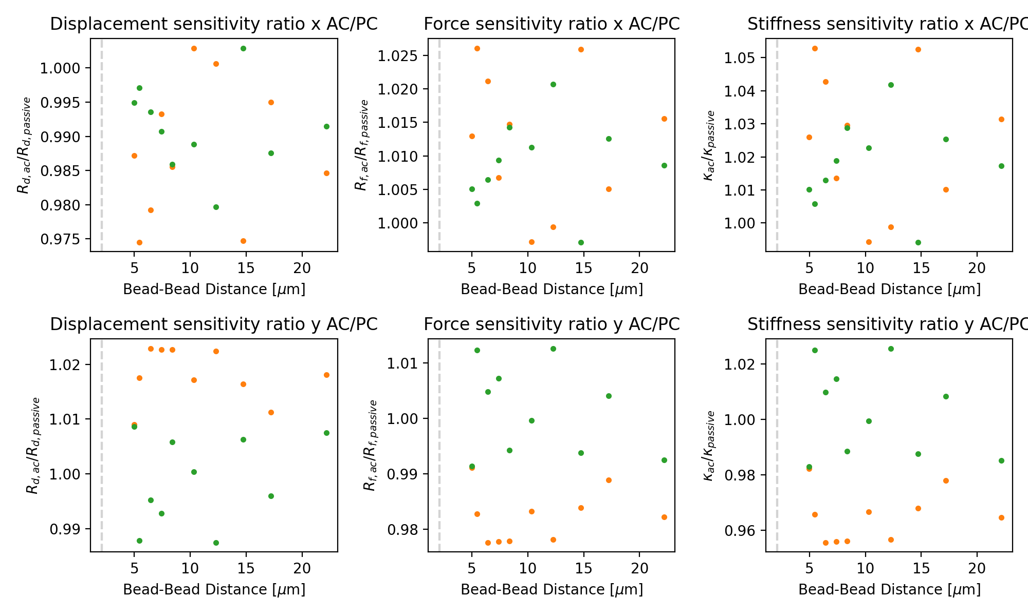
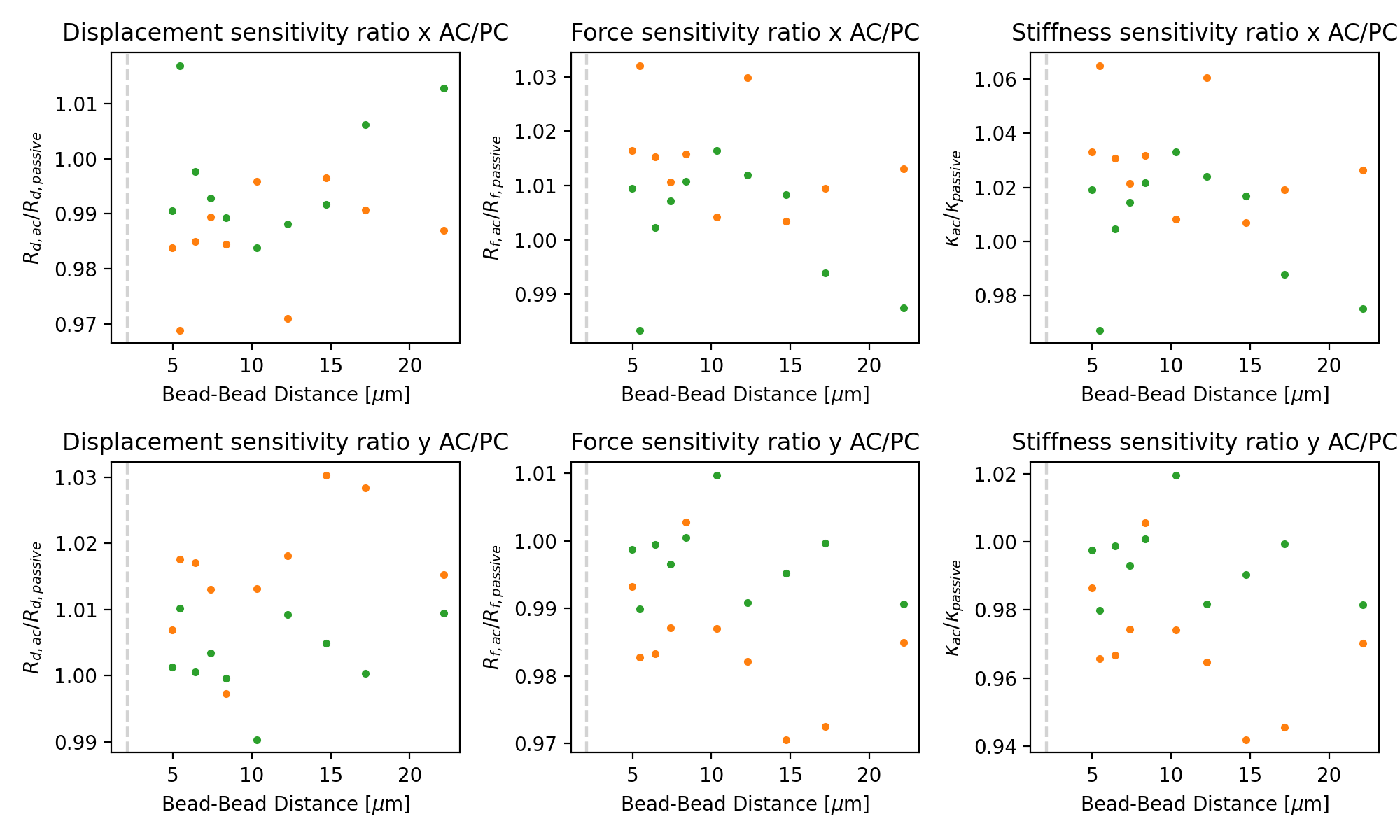
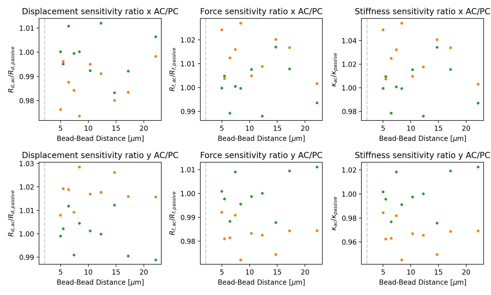
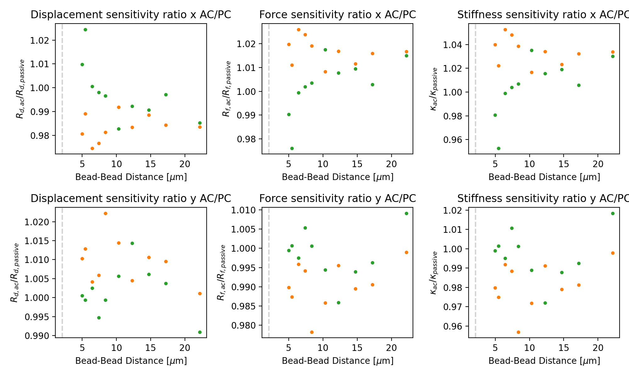
Applying the correction for coupling, we can see that the ratio between active and passive is almost constant.
Some remaining variability is expected as the bead radius (which is subject to variability) and temperature (which isn’t known exactly) impact passive stronger than active:
for exp in experiment:
    dx, dy = extract_distances(exp)
    plt.figure(figsize=(10, 6))

    for trap in (1, 2):
        for ix, axis in enumerate(("x", "y")):
            plt.subplot(2, 3, 1 + 3 * ix)

            # Note that y-oscillations have a different coupling correction than x-oscillations!
            bead_diameter = 2.1
            c = lk.coupling_correction_2d(
                dx, dy, bead_diameter=bead_diameter, is_y_oscillation=True if axis == "y" else False
            )

            ac = extract_parameter(exp, "active", f"{trap}{axis}", "Rd")
            pc = extract_parameter(exp, "passive", f"{trap}{axis}", "Rd")
            plt.plot(dx, ac * c / pc, f"C{trap}.")
            plt.axvline(bead_diameter, color="lightgray", linestyle="--")
            plt.xlabel(r"Bead-Bead Distance [$\mu$m]")
            plt.ylabel("$R_{d, ac} / R_{d, passive}$")
            plt.title(f"Displacement sensitivity ratio {axis} AC/PC")

            plt.subplot(2, 3, 2 + 3 * ix)
            ac = extract_parameter(exp, "active", f"{trap}{axis}", "Rf")
            pc = extract_parameter(exp, "passive", f"{trap}{axis}", "Rf")
            plt.plot(dx, ac / c / pc, f"C{trap}.")
            plt.axvline(bead_diameter, color="lightgray", linestyle="--")
            plt.xlabel(r"Bead-Bead Distance [$\mu$m]")
            plt.ylabel("$R_{f, ac} / R_{f, passive}$")
            plt.title(f"Force sensitivity ratio {axis} AC/PC")

            plt.subplot(2, 3, 3 + 3 * ix)
            ac = extract_parameter(exp, "active", f"{trap}{axis}", "kappa")
            pc = extract_parameter(exp, "passive", f"{trap}{axis}", "kappa")
            plt.plot(dx, ac / c**2 / pc, f"C{trap}.", label=f"{trap}{axis}")
            plt.axvline(bead_diameter, color="lightgray", linestyle="--")
            plt.xlabel(r"Bead-Bead Distance [$\mu$m]")
            plt.ylabel(r"$\kappa_{ac} / \kappa_{passive}$")
            plt.title(f"Stiffness sensitivity ratio {axis} AC/PC")

            plt.tight_layout()