8. Kymotracking

Download this page as a Jupyter notebook

Kymographs are a vital tool in understanding binding events on DNA. They are generated using one-dimensional scans over time. Moving particles can then be seen moving along the spatial coordinate in time. It is often desired to to track the position of such particles in time. Pylake comes with a few features that enable you to do so.

8.1. Performing the tracking

Performing Kymotracking is usually performed in two steps. Typically, there is an image processing step, following by a tracing step, where the actual traces are found.

8.2. Using the greedy algorithm

First, we need to get an image to perform the tracing on. Let’s grab a kymograph from a Bluelake file:

file = lk.File('kymograph.h5')
name, kymo = file.kymos.popitem()

We can extract the image data with one of the _image commands:

data = kymo.green_image

Let’s have a look at what it looks like:

plt.imshow(data, aspect="auto", vmax=5)

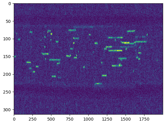
What we also see is that we can clearly see the bead edges in the kymograph. Let’s only take a subsection of the kymograph, to make sure that we don’t get any spurious line detections that come from the bead edges. We only use the 70th to the 220th pixel.

>>> data = data[70:220, :]

If we zoom in a bit, we can see that our traces in this image are about 3 pixels wide, so let’s set this as our line_width. Note that we invoked plt.colorbar() to add a little color legend here.

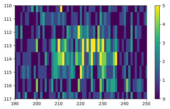
The peaks have an intensity of about 3-7 photon counts, whereas the background fluctuates around 0-2. Let’s set our pixel_threshold to 3. We also see that sometimes, a particle momentarily disappears. To still connect these in a single trace, we want to allow for some gaps in the connection step. Let’s use a window size of 6 in this test. Running the algorithm is easy using the function track_greedy():

traces = lk.track_greedy(data, line_width=3, pixel_threshold=3, window=6)

The result of tracking is a list of kymograph traces:

>>> print(len(traces))  # the number of traces found in the kymo
745

Sometimes, we can have very short spurious traces. To remove these from the list of detected traces we can use filter_lines(). To omit all traces with fewer than 4 detected points, we can invoke:

>>> traces = lk.filter_lines(traces, 3)

We can get the determined time and coordinate indices of these traces from the time_idx and coordinate_idx attributes. Let’s plot the first trace:

plt.plot(traces[0].time_idx, traces[0].coordinate_idx)

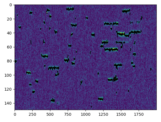
Plotting all the detected traces is also quite easy by iterating over the list of traces:

plt.imshow(data, aspect="auto", vmax=5)
for trace in traces:
    plt.plot(trace.time_idx, trace.coordinate_idx)

Once we are happy with the traces found by the algorithm, we may still want to refine them. Since the algorithm finds traces by determining local peaks and stringing these together, it is possible that some scan lines in the kymograph don’t have an explicit point on the trace associated with them. Using refine_lines_centroid() we can refine the traces found by the algorithm. This function interpolates the lines such that each time point gets its own point on the trace. Subsequently, these points are then refined using a brightness weighted centroid. Let’s perform line refinement and plot the longest trace:

longest_trace_idx = np.argmax([len(trace) for trace in traces])  # Get the longest trace

refined = lk.refine_lines_centroid(traces, line_width=3)

plt.plot(refined[longest_index].time_idx, refined[longest_index].coordinate_idx, '.')
plt.plot(traces[longest_index].time_idx, traces[longest_index].coordinate_idx, '.')
plt.legend(["Post refinement", "Pre-refinement"])
plt.ylabel('Position [pixels]')
plt.xlabel('Time [pixels]')

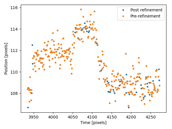
We can see now that a few points were added post refinement (shown in blue). The others remain unchanged, since we used the same line_width.

Fortunately, the signal to noise level in this kymograph is quite good. In practice, when the signal to noise is lower, one will have to resort to some fine tuning of the algorithm parameters over different regions of the kymograph to get an acceptable result.

Note that the determined time and coordinates of the traces and coordinates are defined in pixels and therefore need to be converted to actual time and position using the line time and pixel size of the kymograph. We can get the time between frames directly from the kymograph as Kymo.line_time_seconds and the pixel size as Kymo.pixelsize_um. This allows conversion from pixels back to position.

8.3. Using the kymotracker widget

Using the algorithm purely by function calls can be challenging if not all parts of the kymograph look the same or when the signal to noise ratio is somewhat low. To help with this, we included a kymotracking widget that can help you track subsections of the kymograph and iteratively tweak the algorithm parameters as you do so. You can open this widget by invoking the following command:

kymowidget = lk.KymoWidgetGreedy(data)

You can optionally also pass algorithm parameters when opening the widget:

KymoWidgetGreedy(data, axis_aspect_ratio=2, min_length=4, pixel_threshold=3, window=6, sigma=1.4)

Traced lines are accessible through the .lines property:

>>> lines = kymowidget.lines
KymoLineGroup(N=199)

For more information on its use, please see the example Analyzing Cas9 binding to DNA.

8.4. Using the lines algorithm

The second algorithm present is an algorithm that works purely on signal derivative information. It works by blurring the image, and then performing sub-pixel accurate line detection. It can be a bit more robust to low signal levels, but is generally less temporally and spatially accurate due to the blurring involved:

traces = lk.track_lines(data, line_width=3, max_lines=50)

The interface is mostly the same, aside from an extra required parameter named max_lines which indicates the maximum number of lines we want to detect.

8.5. Extracting summed intensities

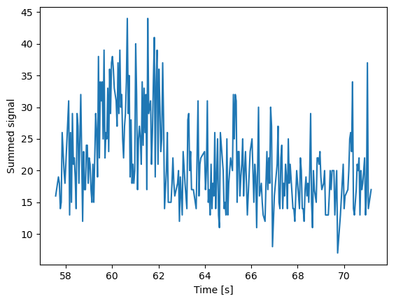
Sometimes, it can be desirable to extract pixel intensities in a region around our kymograph trace. We can quite easily extract these using the method sample_from_image(). For instance, if we want to sum the pixels in a 9 pixel area around the longest kymograph trace, we can invoke:

plt.figure()
longest_trace_idx = np.argmax([len(trace) for trace in traces])
longest_trace = traces[longest_trace_idx]
plt.plot(np.array(longest_trace.time_idx) * kymo.line_time_seconds, longest_trace.sample_from_image(num_pixels=5))
plt.xlabel('Time [s]')
plt.ylabel('Summed signal')

Here num_pixels is the number of pixels to sum on either side of the trace. Note that data has to be the same image that the trace was based on.

8.6. Exporting kymograph traces

Exporting kymograph traces to csv files is easy. Just invoke save on the returned value:

traces.save("traces.csv")

By default, this saves the kymograph in pixel coordinates. We can also save calibrated coordinates and photon counts by passing a calibration factor for the x-axis and y-axis and a width in pixels to sum counts over:

traces.save("traces_calibrated.csv", dt=kymo.line_time_seconds, dx=kymo.pixelsize_um, sampling_width=3)

8.7. How the algorithms work

track_greedy()

The first method implemented for performing such a tracking is based on [SK05][MPP16]. It starts by performing peak detection, performing a grey dilation on the image, and detection which pixels remain unchanged. Peaks that fall below a certain intensity threshold are discarded. Since this peak detection operates at a pixel granularity, it is followed up by a refinement step to attain subpixel accuracy. This refinement is performed by computing an offset from a brightness-weighted centroid in a small neighborhood w around the pixel.

\[offset = \frac{1}{m} \sum_{i^2 < w^2} i I(x + i)\]

Where m is given by:

\[m = \sum_{i^2 < w^2} I(x + i)\]

After peak detection the feature points are linked together using a forward search analogous to [MPP16]. This is in contrast with the linking algorithm in [SK05] which uses a graph-based optimization approach. This linking step traverses the kymograph, tracing particles starting from each frame.

• The algorithm starts at time frame one (the first pixel column).
• It selects the peak with the highest pixel intensity and initiates the first trace.
• Next, it evaluates the subsequent frame, and computes a connection score for each peak in the next frame (to be specified in more detail later).
• If a peak is found with an acceptable score, the peak is added to the trace.
• When no more candidates are available we look in the next window frames to see if we can find an acceptable peak there, following the same procedure.
• Once no more candidates are found in the next window frames, the trace is terminated and we proceed by initiating a new trace from the peak which is now the highest.
• Once there are no more peaks in the frame from which we are currently initiating traces, we start initiating traces from the next frame. This process is continued until there are no more peaks left to trace.

The score function is based on a prediction of where we expect future peaks. Based on the peak location of the tip of the trace x and a velocity v, it computes a predicted position over time. The score function assumes a Gaussian uncertainty around that prediction, placing the mean of that uncertainty on the predicted extrapolation. The width of this uncertainty is given by a base width (provided as sigma) and a growing uncertainty over time given by a diffusion rate. This results in the following model for the connection score.

\[S(x, t) = N\left(x + v t, \sigma_{base} + \sigma_{diffusion} \sqrt{t}\right).\]

Here N refers to a normal distribution. In addition to the model, we also have to set a cutoff, after which we deem peaks to be so unlikely to be connected that they shouldn’t be. By default, this cutoff is set at two sigma. Scores outside this cutoff are set to zero which means they will not be accepted as a new point.

track_lines()

The second algorithm is an algorithm that looks for curvilinear structures in an image. This method is based on sections 1, 2 and 3 from [Ste98]. This method attempts to find lines purely based on the derivatives of the image. It blurs the image based with a user specified line width and then attempts to find curvilinear sections.

Based on the second derivatives of the blurred image, a Hessian matrix is constructed. This Hessian matrix is decomposed using an eigenvector decomposition to obtain the perpendicular and tangent directions to the line. To attain subpixel accuracy, the maximum is computed perpendicular to the line using a local Taylor expansion. This expansion provides an offset on the pixel position. When this offset falls within the pixel, then this point is considered to be part of a line. If it falls outside the pixel, then it is not a line.

This provides a narrow mask, which can be traced. Whenever ambiguity arises on which point to connect next, a score comprised of the distance to the next subpixel minimum and angle between the successive normal vectors is computed. The candidate with the lowest score is then selected.

Since this algorithm is specifically looking for curvilinear structures, it can have issues with structures that are more blob-like (such as short-lived fluorescent events) or diffusive traces, where the particle moves randomly rather than in a uniform direction.