1.1. Kinesin Walking on Microtubule
Download this page as a Jupyter notebook
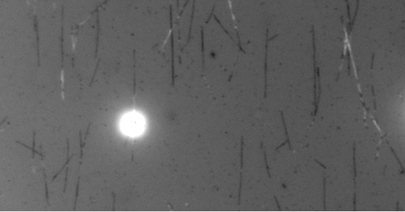
In this assay we had microtubules on the surface. We trapped beads with kinesin (molecular motor) and had ATP inside the assay. As we lowered the kinesin-coated beads on top of a microtubule, it attached and started stepping on them. Kinesins were pulling the bead out of the center of the trap and thus increasing the force on the bead. At one point the kinesins couldn’t keep up with this increased force and the bead construct snapped back to its original position.
After this, the cycles starts again with kinesins pulling the bead out of the center of the trap.
With IRM, you can see unlabeled microtubules and the kinesin-coated bead on top of one of them.
To see and characterize this behavior, we need to have the following plots:
Plot force versus time
Plot the displacement of the bead from the center of the trap over time
Download the files with download_from_doi():
lk.download_from_doi("10.5281/zenodo.12666579", "data")
Open the File:
file = lk.File("data/stepping_open_loop.h5")
1.1.1. Force versus Time
Extract the raw data:
force1x = file["Force HF"]["Force 1x"]
force1y = file["Force HF"]["Force 1y"]
Plot force in x and y:
plt.figure(figsize=(13, 5))

plt.subplot(2, 1, 1)
force1x.plot()
plt.ylabel("Force X (pN)")

plt.subplot(2, 1, 2)
force1y.plot()
plt.ylabel("Force Y (pN)");
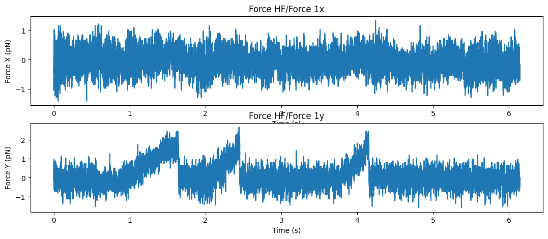
We can clearly see that the bead was moving in the y direction, so for now we’re just going to work with that. A different example shows how to deal with a bead moving at an angle (e.g. at 45 degrees).
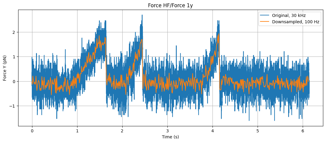
For now, let’s also down-sample the force data to 100 Hz and plot the two together.
Downsample the y force data using downsampled_by():
downsampled_rate = 100  # Hz

sample_rate = force1y.sample_rate
downsampling_factor = int(sample_rate / downsampled_rate)
force1x_downsamp = force1x.downsampled_by(downsampling_factor)
force1y_downsamp = force1y.downsampled_by(downsampling_factor)
The two sampling rates are:
>>> print(f"Original sampling rate is {sample_rate} Hz")
>>> print(f"Downsampled rate is {downsampled_rate} Hz")

Original sampling rate is 30000 Hz
Downsampled rate is 100 Hz
Plot the original force and the downsampled rate:
plt.figure(figsize=(13, 5))

force1y.plot(label="Original, 30 kHz")
force1y_downsamp.plot(label="Downsampled, 100 Hz")
plt.ylabel("Force Y (pN)")
plt.legend()
plt.grid()
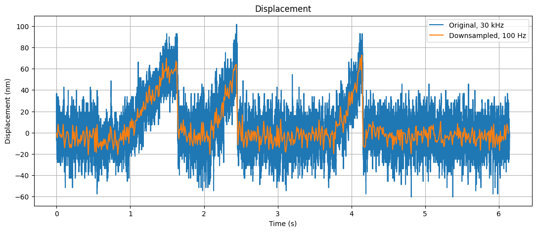
1.1.2. Displacement versus Time
We need to convert the force to displacement, which we can do with the following formula:
where F is the force and k is the trap stiffness. Force we already have, we need to get stiffness.
Get stiffness from force calibration:
kx = force1x.calibration[0]["kappa (pN/nm)"]
ky = force1y.calibration[0]["kappa (pN/nm)"]
The stiffness values are:
>>> print(kx)  # this is in pN/nm
>>> print(ky)  # this is in pN/nm
0.019126295617530483
0.02648593456747345
Calculate and plot displacement versus time:
displacement = force1y / ky
displacement_downsampled = force1y_downsamp / ky

plt.figure(figsize=(13, 5))
displacement.plot(label="Original, 30 kHz")
displacement_downsampled.plot(label="Downsampled, 100 Hz")
plt.title("Displacement")
plt.ylabel("Displacement (nm)")
plt.legend()
plt.grid()
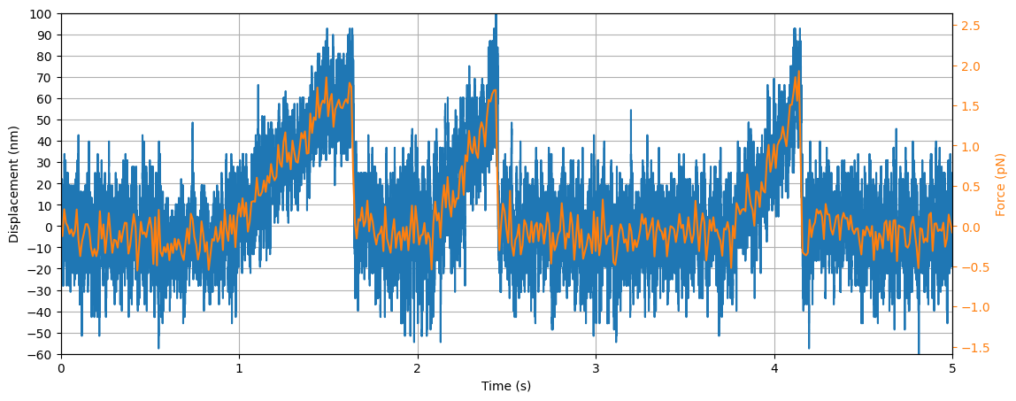
1.1.3. Distance and Force versus Time on Same Graph
Plot:
fig, ax1 = plt.subplots(figsize=(13, 5))
displacement.plot(label="Original, 30 kHz")
ax1.set_ylabel("Displacement (nm)")
ax1.set_yticks(range(-60, 110, 10))
ax1.set_title("")
ax1.grid()

# create another axis
ax2 = ax1.twinx()

ax2.plot(
    force1y_downsamp.seconds,
    force1y_downsamp.data,
    color="tab:orange",
    label="Downsampled, 100 Hz"
)
ax2.set_ylabel("Force (pN)", color="tab:orange")
ax2.tick_params("y", colors="tab:orange")

# Here we just make sure that both the displacement and the force axis have the same limits
y_limits = np.array([-60, 100])
y_lim2 = y_limits * ky

ax1.set_ylim(y_limits)
ax2.set_ylim(y_lim2)
ax1.set_xlim([0, 5])
1.1.4. X vs Y Position of the Bead
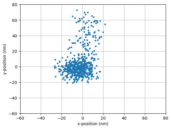
To get an idea in which direction the microtubule was oriented, which direction the force was applied, we plot the (x,y) position of the bead:
plt.plot(force1x_downsamp.data / kx, force1y_downsamp.data / ky, ".")
plt.xlim([-60, 80])
plt.ylim([-60, 80])

plt.xlabel("x-position (nm)")
plt.ylabel("y-position (nm)")

plt.grid()