3. Twistable Worm-Like-Chain Fitting
Download this page as a Jupyter notebook
In this notebook, we analyze force extension data of DNA over its full range of structural transitions under mechanical stress (0 - 60 pN). The twistable worm-like chain model (tWLC) takes twisting deformations on the DNA double helix into account. Here we will use this model to describe the mechanical response of DNA at such high forces.
Download the files with download_from_doi():
lk.download_from_doi("10.5281/zenodo.12668419", "data")
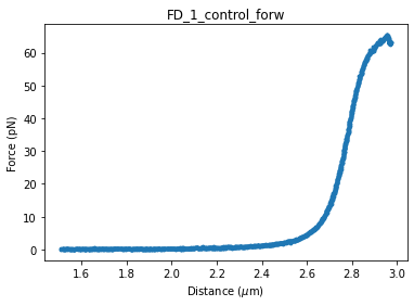
Let’s load and plot the data first:
file = lk.File("data/twlc_data.h5")
fd_curve = file.fdcurves["FD_1_control_forw"]
fd_curve.plot_scatter()
3.1. Set up a basic model first
We clearly see that the force starts levelling out at high forces in the data. We’ll need something rather complex in order to capture this behavior. The twistable worm-like chain (tWLC) model can describe the untwisting behavior of DNA that becomes apparent in the 30-60 pN force range. However, the model’s complexity also incurs some challenges.
Parameter estimation typically begins from an initial guess, and if this initial guess is bad, it can get stuck at an estimated set of parameters that are suboptimal, a so-called local optimum. One way to mitigate this, is to start with better initial values.
In this notebook, we fit the region before the force begins levelling out (i.e. 30 pN) first with a regular worm-like chain model and then use those estimates as initial guesses to fit the tWLC model.
Depending on your experiments, small offsets can be present in the data. For instance, the bead diameter may vary
slightly from experiment to experiment, or the force may have experienced some drift. We incorporate an offset in
both distance and force to compensate for small offsets that may exist in the data. Let’s set up the Odijk worm-like
chain model using the function ewlc_odijk_force() and create the fit:
m_odijk = lk.ewlc_odijk_force("DNA").subtract_independent_offset() + lk.force_offset("DNA")
fit_odijk = lk.FdFit(m_odijk)
Considering that this model only describes the force-extension behaviour at low forces (0.1 - 30 pN), we have to extract the data that is relevant to us. We can obtain this data from the force-distance curve as follows:
force = fd_curve.f.data
distance = fd_curve.d.data
We only wish to use the forces below 30, so we filter the data according to this requirement:
mask = force < 30
distance = distance[mask]
force = force[mask]
Now we are ready to add this data to the fit using add_data(), but first, we must constrain the distance offset to help the fitting,
as this provides a lot of additional freedom in the model:
fit_odijk.add_data("Inverted Odijk", force, distance)
fit_odijk["DNA/d_offset"].upper_bound = 0.01
fit_odijk["DNA/d_offset"].lower_bound = -0.01
And fit() the model:
>>> fit_odijk.fit()

Fit
  - Model: DNA(x-d)_with_DNA
  - Equation:
      f(d) = argmin[f](norm(DNA.Lc * (1 - (1/2)*sqrt(kT/(f*DNA.Lp)) + f/DNA.St)-(d - DNA.d_offset))) + DNA.f_offset

  - Data sets:
    - FitData(Inverted Odijk, N=959)

  - Fitted parameters:
    Name                  Value  Unit      Fitted      Lower bound    Upper bound
    ------------  -------------  --------  --------  -------------  -------------
    DNA/d_offset    -0.00601252  [au]      True              -0.01           0.01
    DNA/Lp          44.2558      [nm]      True               0            100
    DNA/Lc           2.80085     [micron]  True               0            inf
    DNA/St        1714.56        [pN]      True               0            inf
    kT               4.11        [pN*nm]   False              0              8
    DNA/f_offset     0.0392458   [pN]      True              -0.1            0.1
3.2. Set up the twistable worm like chain model
By default, the twlc_distance() model provided with pylake outputs the distance as a function of force.
However, we typically want to fit force as a function of distance.
To achieve this, we can invert the model using its invert() function at the cost of slowing down the fit.
Alternatively, we have a faster way of achieving this in pylake, by using the dedicated twlc_force() model:
m_dna = lk.twlc_force("DNA").subtract_independent_offset() + lk.force_offset("DNA")
fit_twlc = lk.FdFit(m_dna)
3.3. Load the full data into the model
In the plot showing the data, we could see that there is a small transition event at the end of the Fd curve. The model will not be able to capture this behaviour and therefore it is best to remove this section prior to fitting:
force = fd_curve.f.data
distance = fd_curve.d.data
mask = distance < 2.88
distance = distance[mask]
force = force[mask]
Now we can load the data into the model:
fit_twlc.add_data("Twistable WLC", force, distance)
We could add more datasets in a similar manner, but in this example, we only fit a single model. Let’s load the parameters from our previous fit to use them as initial guesses for this one. We also fix the twist rigidity and critical force to values from literature (analogous to Broekmans et al. “DNA twist stability changes with magnesium (2+) concentration.” Physical Review Letters 116, 258102 (2016)):
fit_twlc.update_params(fit_odijk)

# Fix twist rigidity and critical force to literature values.
fit_twlc["DNA/C"].value = 440
fit_twlc["DNA/C"].fixed = True
fit_twlc["DNA/Fc"].value = 30.6
fit_twlc["DNA/Fc"].fixed = True
3.4. Fit the model
Considering that the tWLC model is more difficult to evaluate, this may take a while. This is also why we choose to enable verbose output:
>>> fit_twlc.fit(verbose=2)
>>> plt.show()

   Iteration     Total nfev        Cost      Cost reduction    Step norm     Optimality
       0              1         2.4384e+02                                    2.81e+05
       1              2         4.4649e+01      1.99e+02       6.84e+00       1.14e+04
       2              3         4.3820e+01      8.29e-01       5.79e+01       4.67e+03
       3              4         4.3756e+01      6.46e-02       1.36e+01       2.16e+02
       4              5         4.3755e+01      8.30e-04       3.92e+00       9.48e+00
       5              6         4.3755e+01      1.29e-06       7.15e-02       5.84e-02
       6              7         4.3755e+01      5.81e-09       3.60e-02       1.86e-02
`ftol` termination condition is satisfied.
Function evaluations 7, initial cost 2.4384e+02, final cost 4.3755e+01, first-order optimality 1.86e-02.
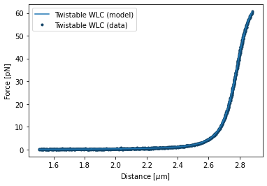
3.5. Plotting the results
After fitting we can plot our results and print our parameters by invoking plot() and params respectively:
fit_twlc.plot()
plt.xlabel("Distance [$\\mu$m]")
plt.ylabel("Force [pN]");
We can also show the parameters:
>>> fit_twlc.params

Name                  Value  Unit        Fitted      Lower bound    Upper bound
------------  -------------  ----------  --------  -------------  -------------
DNA/d_offset    -0.00605829  [au]        True              -0.01           0.01
DNA/Lp          43.2315      [nm]        True               0            100
DNA/Lc           2.80289     [micron]    True               0            inf
DNA/St        1761.79        [pN]        True               0            inf
DNA/C          440           [pN*nm**2]  False              0           5000
DNA/g0        -579.909       [pN*nm]     True           -5000              0
DNA/g1          17.6625      [nm]        True               0           1000
DNA/Fc          30.6         [pN]        False              0             50
kT               4.11        [pN*nm]     False              0              8
DNA/f_offset     0.0295708   [pN]        True              -0.1            0.1
These seem to agree well with what’s typically found for dsDNA.