10.4. Diode calibration

Download this page as a Jupyter notebook

When calibrating, it is important to take into account the characteristics of the sensor used to measure the data.

Depending on the sensor in your system, and whether it was pre-calibrated you may need to consider a few extra steps in the calibration procedure. We will illustrate this on a small dataset:

lk.download_from_doi("10.5281/zenodo.7729823", "test_data")
f = lk.File("test_data/noise_floor.h5")

Let’s grab a calibration item from the file and check whether it was a full calibration by checking its kind property. If this returns "Active" or "Passive", it means that it was a full calibration, meaning it will have information about the diode in the calibration item:

>>> calibration_item = f.force1x.calibration[0]
... calibration_item.kind
'Passive'

If the last item was a full calibration, we can check whether this system has a calibrated diode by checking the fitted_diode property:

>>> calibration_item.fitted_diode
False

In this case the property is False, which means the diode was not fitted during the calibration. In other words, a pre-calibrated diode was used. We can extract the diode calibration model as follows:

>>> diode_calibration = calibration_item.diode_calibration
... diode_calibration
DiodeCalibrationModel()

This model describes the relation between trap power and the sensor parameters. To use this model, call it with total trap power to determine the diode parameters at that power level.

>>> diode_params = diode_calibration(f["Diagnostics"]["Trap power 1"])
... diode_params
{'fixed_diode': 14829.480905511606, 'fixed_alpha': 0.4489251910346808}

These parameter values can be used directly with calibrate_force(). A convenient way to do this is to grab the calibration parameters of a previous calibration, and only update the diode calibration parameters. Below is an example of how to do this with a dict union using the | operator:

>>> params = calibration_item.calibration_params()
... # replace the 'fixed_diode' and 'fixed_alpha' values in params
... # with the corresponding values from diode_params and return a new dict
... updated_params = params | diode_params
... print(updated_params)
{'num_points_per_block': 200,
 'sample_rate': 100000,
 'excluded_ranges': [],
 'fit_range': (10.0, 23000.0),
 'bead_diameter': 4.34,
 'rho_bead': 1060.0,
 'rho_sample': 997.0,
 'viscosity': 0.000941,
 'temperature': 22.58,
 'fixed_alpha': 0.4489251910346808,
 'fixed_diode': 14829.480905511606,
 'fast_sensor': False,
 'axial': False,
 'hydrodynamically_correct': True,
 'active_calibration': False}

We can see that this updated the fixed diode parameters.

Note

Each sensor has its own diode characteristic. If you are calibrating multiple traps with pre-calibrated diodes, you will need to provide the correct diode parameters for each trap. Each sensor has their own diode calibration values!

We can calibrate with these parameters directly by unpacking this dictionary into the calibrate_force() function:

volts = f.force1x / f.force1x.calibration[0].force_sensitivity

calibration = lk.calibrate_force(volts.data, **updated_params)
calibration.plot()

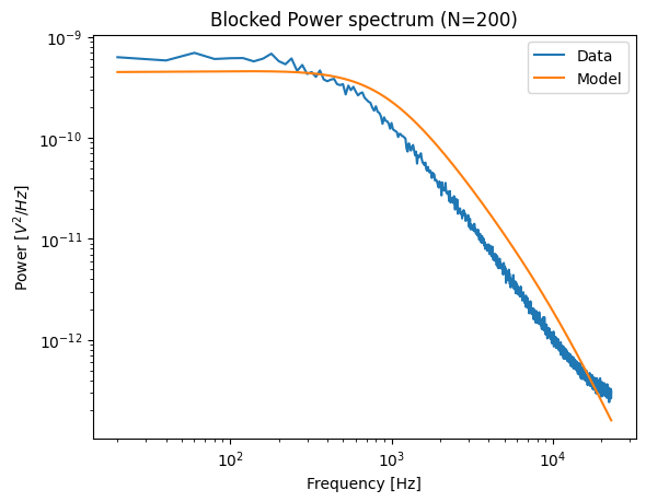
Unfortunately, in this case, we also have a noise floor to contend with, so we should restrict the fitting range as well (for more information about this, see the section on noise floors).

To automatically determine a reasonable fit range, we can pass the extra parameter corner_frequency_factor to calibrate_force. This will iterative fit the power spectrum and constrain the fitted part of the spectrum to a region around the corner frequency given up to a fraction of the corner frequency. An empirically determined reasonable value to use here is 4:

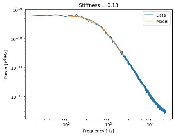
calibration = lk.calibrate_force(volts.data, **updated_params, corner_frequency_factor=4)
calibration.plot(data_range=(5, 23000))
plt.title(f"Stiffness = {calibration.stiffness:.2f}");

Note that if adaptive fitting ranges were used in Bluelake, then the user defined initial fitting ranges and used corner frequency factor can be found in initial_fit_range and corner_frequency_factor, while the used fitting range can be found in fit_range.

In this case, we also passed a custom data_range to show more of the original power spectral data.

Note

Automatic fitting ranges can only be used in conjunction with a calibrated diode. The reason for this is that this method will trim those parts of the power spectrum that are needed for estimating the diode parameters when the corner frequency is low.

We can also restrict the upper bound of the fitting range manually to approximately four times the corner frequency:

volts = f.force1x / f.force1x.calibration[0].force_sensitivity

updated_params = updated_params | {"fit_range": [100, 2300]}
calibration = lk.calibrate_force(volts.data, **updated_params)
calibration.plot(data_range=(5, 23000))
plt.title(f"Stiffness = {calibration.stiffness:.2f}");

To judge whether the noise floor has been sufficiently truncated, you can play with the upper limit of the fit range and see if the corner frequency no longer changes.

10.4.1. When to use calibrated diode parameters

Using a calibrated diode is critical when the corner frequency is close to or higher than the diode frequency. When the corner frequency is very high, the estimation of the model parameters can fail despite the fit looking good.

In this data, the corner frequency is low, therefore using the diode parameters is not strictly necessary:

>>> calibration.corner_frequency
531.0129872280306

Removing fixed_diode and fixed_alpha from the calibration arguments (by setting them to None) results in almost no change in this case:

updated_params = updated_params | {"fixed_alpha": None, "fixed_diode": None, "fit_range": [100, 2300]}
calibration = lk.calibrate_force(volts.data, **updated_params)
calibration.plot()
plt.title(f"Stiffness: {calibration.stiffness:.2f}");

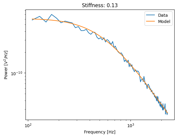
As we can see, the stiffness is pretty much the same in this case.