Hydrodynamically correct model
Download this page as a Jupyter notebook
While the idealized model of the bead motion is sometimes sufficiently accurate, it neglects inertial and hydrodynamical effects of the fluid and bead(s).
The frictional forces applied by the viscous environment to the bead are proportional to the bead’s velocity relative to the fluid. The idealized model is based on the assumption that the bead’s relative velocity is constant; there is no dynamical change of the fluid motion around the bead. In reality, when the bead moves through the fluid, the frictional force between the bead and the fluid depends on the past motion, since that determines the fluid’s current motion. For a stochastic process such as Brownian motion, constant motion is not an accurate assumption. In addition, the bead and the surrounding fluid have their own mass and inertia, which are also neglected in the idealized model.
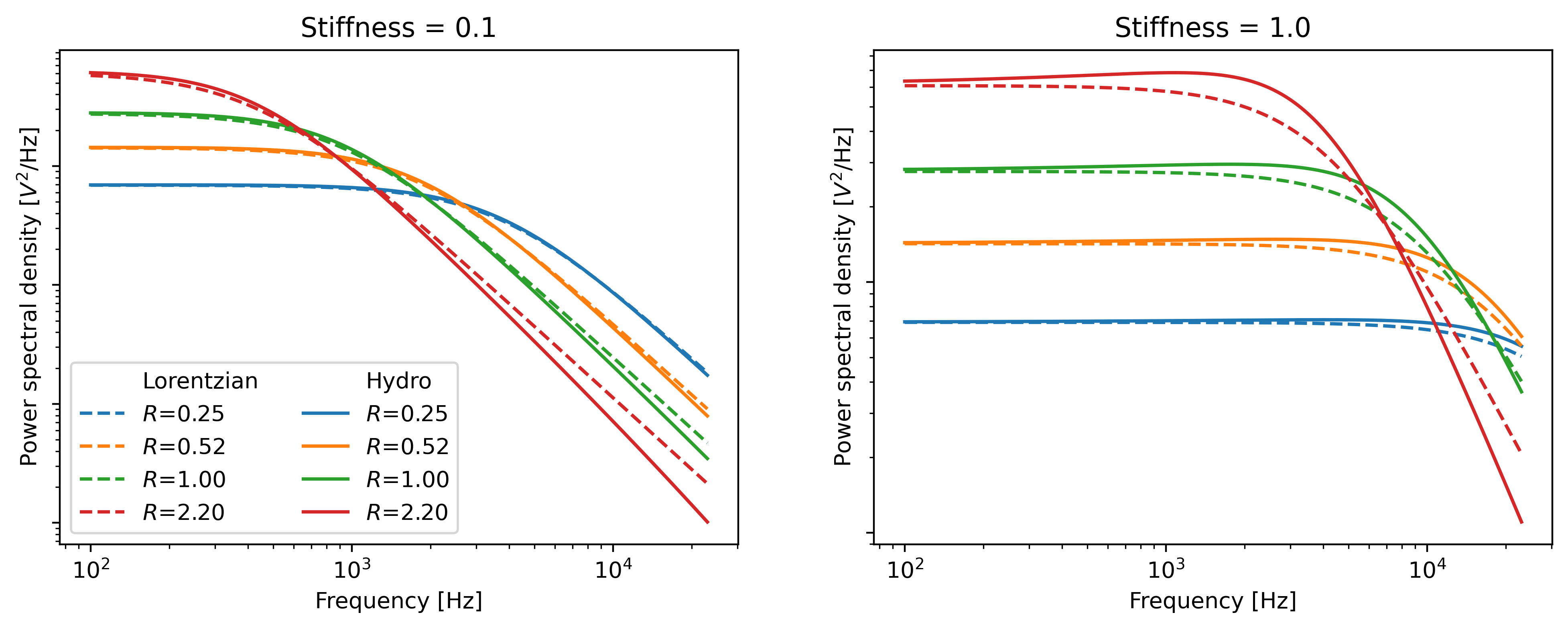
Together, the non-constant relative velocity and the inertial effects result in frequency-dependent frictional forces that a more accurate hydrodynamically correct model takes into account. These effects are strongest at higher frequencies, and for larger bead diameters.
The figure below shows the difference between the hydrodynamically correct model (solid lines) and the idealized Lorentzian model (dashed lines) for various bead sizes. It can be seen that for large bead sizes and higher trap powers the differences can be substantial.
Fast sensor measurement
Note
The following section only applies to instruments which contain fast PSDs.
When fitting a power spectrum, one may ask the question: “Why does the fit look good if the model is bad?” The answer to this lies in the model that is used to capture the parasitic filtering effect. When the parameters of this model are estimated, they can “hide” the mis-specification of the model.
Fast detectors have the ability to respond much faster to incoming light resulting in no visible filtering effect in the frequency range we are fitting. This means that for a fast detector, we do not need to include such a filtering effect in our model and see the power spectrum for what it really is.
We can omit this effect by passing fast_sensor=True to the calibration models or to calibrate_force().
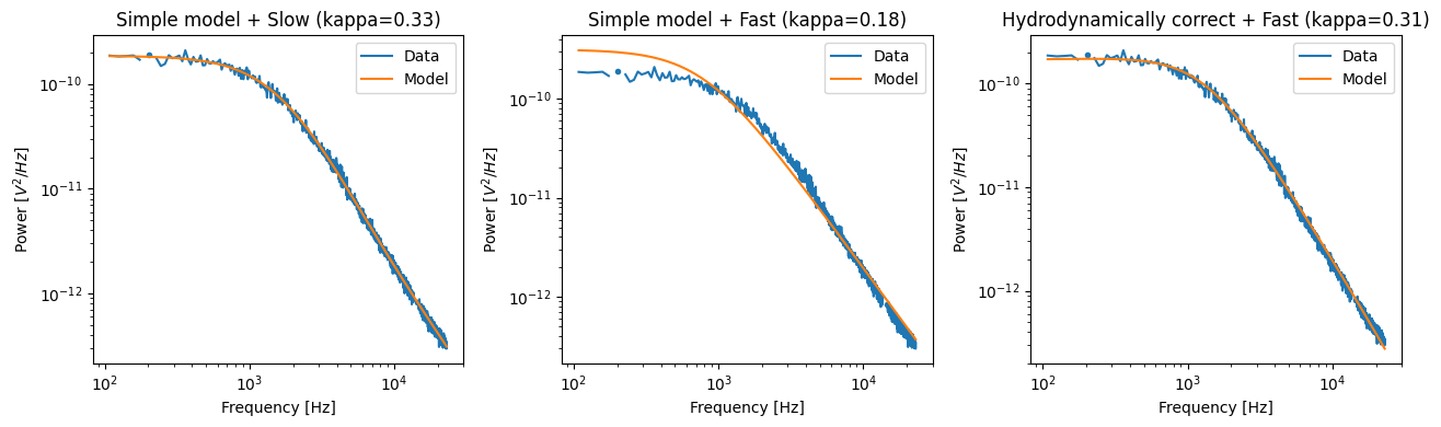
Note however, that this makes using the hydrodynamically correct model critical, as the simple model doesn’t actually capture the data very well.
The following example data acquired on a fast sensor will illustrate why:
filenames = lk.download_from_doi("10.5281/zenodo.7729823", "test_data")
f = lk.File("test_data/fast_measurement_25.h5")

# Decalibrate the force data
volts = f.force2y / f.force2y.calibration[0].force_sensitivity

shared_parameters = {
    "force_voltage_data": volts.data,
    "bead_diameter": 4.38,
    "temperature": 25,
    "sample_rate": volts.sample_rate,
    "fit_range": (1e2, 23e3),
    "num_points_per_block": 200,
    "excluded_ranges": ([190, 210], [13600, 14600])
}

plt.figure(figsize=(13, 4))
plt.subplot(1, 3, 1)
fit = lk.calibrate_force(**shared_parameters, hydrodynamically_correct=False, fast_sensor=False)
fit.plot()
plt.title(f"Simple model + Slow (kappa={fit['kappa'].value:.2f})")
plt.subplot(1, 3, 2)
fit = lk.calibrate_force(**shared_parameters, hydrodynamically_correct=False, fast_sensor=True)
fit.plot()
plt.title(f"Simple model + Fast (kappa={fit['kappa'].value:.2f})")
plt.subplot(1, 3, 3)
fit = lk.calibrate_force(**shared_parameters, hydrodynamically_correct=True, fast_sensor=True)
fit.plot()
plt.title(f"Hydrodynamically correct + Fast (kappa={fit['kappa'].value:.2f})")
plt.tight_layout()
plt.show()
Mathematical background
This section will detail some of the implementational aspects of the hydrodynamically correct model. The following equation accounts for a frequency dependent drag [TolicNorrelykkeSchafferH+06]:
where the corner frequency is given by:
and \(f_{m, 0}\) parameterizes the time it takes for friction to dissipate the kinetic energy of the bead:
with \(m\) the mass of the bead. Finally, \(\gamma\) corresponds to the frequency dependent drag. For measurements in bulk, far away from a surface, \(\gamma\) = \(\gamma_\mathrm{stokes}\), where \(\gamma_\mathrm{stokes}\) is given by:
Here \(f_{\nu}\) is the frequency at which the penetration depth equals the radius of the bead, \(4 \nu/(\pi d^2)\) with \(\nu\) the kinematic viscosity.
This approximation is reasonable, when the bead is far from the surface.