Passive calibration¶

Download this page as a Jupyter notebook

Passive calibration is also often referred to as thermal calibration and involves calibration without moving the trap or stage. In passive calibration, the Brownian motion of the bead in the trap is analyzed in order to find calibration factors for both the positional detection as well as the force.

To fit passive calibration data, we will use a model based on a number of publications by the Flyvbjerg group [BSF04, BSPW+06, HTNFBS06, TNBSF04]. The Pylake implementation of this model is PassiveCalibrationModel. The most basic form of passive calibration starts by fitting the following equation to the power spectrum:

\[P(f) = \frac{D_\mathrm{measured}}{\pi ^ 2 \left(f^2 + f_c ^ 2\right)} g(f, f_\mathrm{diode}, \alpha) \tag{$\mathrm{V^2/Hz}$}\]

where $D_\mathrm{measured}$ corresponds to the diffusion constant (in $V^2/s$), $f$ the frequency and $f_c$ the corner frequency. The first part of the equation is the same as before and represents the part of the spectrum that originates from the physical motion of the bead. The second term $g$ takes into account the slower response of the position detection system and is given by:

\[g(f, f_\mathrm{diode}, \alpha) = \alpha^2 + \frac{1 - \alpha ^ 2}{1 + (f / f_\mathrm{diode})^2} \tag{$-$}\]

Here $\alpha$ corresponds to the fraction of the signal response that is instantaneous, while $f_\mathrm{diode}$ characterizes the frequency response of the diode. Note that not all sensor types require this second term.

To convert the parameters obtained from this spectral fit to a trap stiffness, the following is computed:

\[\kappa = 2 \pi \gamma_0 f_c \tag{$\mathrm{N/m}$}\]

where $\kappa$ is the estimated trap stiffness.

We can calibrate the position by considering the diffusion of the bead:

\[D_\mathrm{physical} = \frac{k_B T}{\gamma_0} \tag{$\mathrm{m^2/s}$}\]

Here $k_B$ is the Boltzmann constant and $T$ is the local temperature in Kelvin. Comparing this to its measured counterpart in Volts squared per second provides us with the desired calibration factor:

\[R_d = \sqrt{\frac{D_\mathrm{physical}}{D_\mathrm{measured}}} \tag{$\mathrm{m/V}$}\]

The force response $R_f$ can then be computed as:

\[R_f = \kappa R_d \tag{$\mathrm{N/V}$}\]

All three of these quantities depend on the parameter $\gamma_0$, which corresponds to the drag coefficient of a sphere and is given by:

\[\gamma_0 = 3 \pi \eta(T) d \tag{$\mathrm{kg/s}$}\]

where $\eta(T)$ corresponds to the dynamic viscosity [Pa*s] and $d$ is the bead diameter [m].

The effect of temperature¶

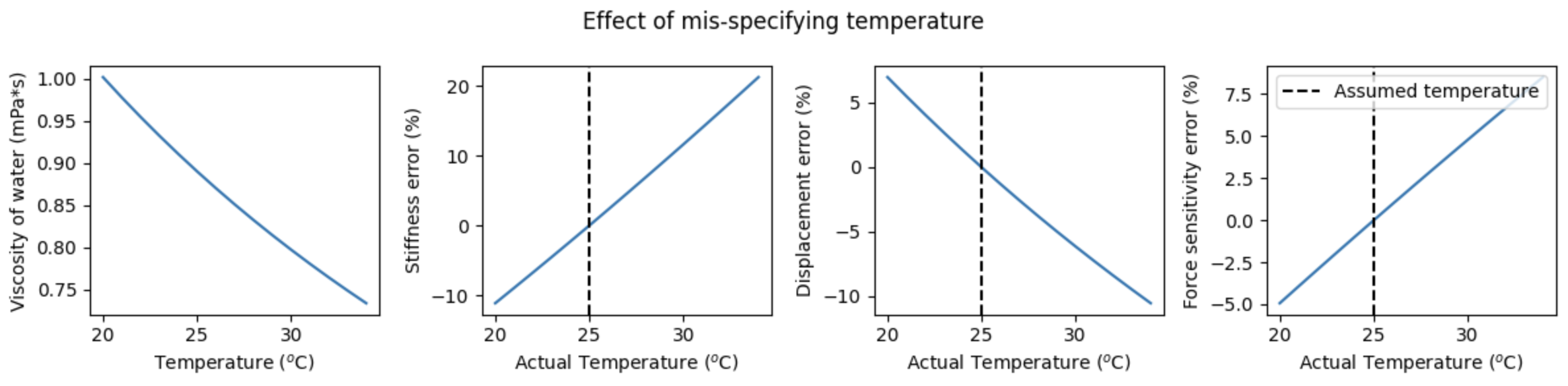
As we can see above, temperature enters the calibration procedure both directly, as well as through the medium viscosity. It is especially the latter that results in large calibration errors when mis-specified.

\[\begin{split}\begin{align} \kappa = 2 \pi \gamma(T) f_c &\propto& \eta(T)\\ R_d = \sqrt{\frac{kT}{\gamma(T)D_\mathrm{volts}}} &\propto& \sqrt{T / \eta(T)}\\ R_f = R_d \kappa &\propto& \sqrt{T \eta(T)} \end{align}\end{split}\]

Mis-specification can lead to errors in calibration. To get a feeling for the magnitude of these errors, we can plot them:

plt.figure(figsize=(12, 3))
temps = np.arange(20, 35)
viscosity_25 = lk.viscosity_of_water(25)
plt.subplot(1, 4, 1)
plt.plot(temps, 1000 * lk.viscosity_of_water(temps))
plt.xlabel("Temperature ($^o$C)")
plt.ylabel("Viscosity of water (mPa*s)")

plt.subplot(1, 4, 2)
viscosities = lk.viscosity_of_water(temps)
kappa_err = 100 * (viscosity_25 / viscosities - 1)
plt.plot(temps, kappa_err)
plt.xlabel("Actual Temperature ($^o$C)")
plt.ylabel("Stiffness error (%)")
plt.axvline(25, linestyle="--", color="k")
plt.tight_layout()

plt.subplot(1, 4, 3)
rd_err = 100 * (np.sqrt((25 + 273.15) / viscosity_25) / np.sqrt((temps + 273.15) / viscosities) - 1)
plt.plot(temps, rd_err)
plt.xlabel("Actual Temperature ($^o$C)")
plt.ylabel("Displacement error (%)")
plt.axvline(25, linestyle="--", color="k")
plt.tight_layout()

plt.subplot(1, 4, 4)
rf_err = 100 * (np.sqrt((25 + 273.15) * viscosity_25) / np.sqrt((temps + 273.15) * viscosities) - 1)
plt.plot(temps, rf_err)
plt.xlabel("Actual Temperature ($^o$C)")
plt.ylabel("Force sensitivity error (%)")
plt.axvline(25, linestyle="--", color="k", label="Assumed temperature")
plt.suptitle("Effect of mis-specifying temperature")
plt.tight_layout()
plt.legend()