Fitting a power spectrum¶

Download this page as a Jupyter notebook

In the previous sections, the physical origin of the power spectrum was introduced. However, there are some additional practical aspects to consider.

Spectral down-sampling¶

So far, we have treated the power spectrum as a simple smooth curve where each frequency corresponds to a given amplitude. What we actually have been looking at is the expected value of the power spectrum. Basically, if you were to average many power spectra, their average would eventually converge to this curve.

In reality, each data point in a power spectrum follows a distribution. The real and imaginary part of the complex spectrum are normally distributed. This spectrum is squared to obtain our power spectrum. As a consequence, the squared magnitude of the power spectrum is exponentially distributed.

This has two consequences:

Fitting the power spectral values directly using a simple least squares fitting routine, we would get very biased estimates. These estimates would overestimate the plateau and corner frequency, resulting in overestimated trap stiffness and force response and an underestimated distance response.
The signal to noise ratio is poor (equal to one [NF10]).

A commonly used method for dealing with this involves data averaging, which trades resolution for an improved signal to noise ratio. By virtue of the central limit theorem, as we average more data, the distribution of the data points becomes more and more Gaussian and therefore more amenable to standard least-squares fitting procedures.

There are two ways to perform such averaging:

The first is to split the time series into windows of equal length, compute the power spectrum for each chunk of data and averaging these. This procedure is referred to as windowing.
The second is to calculate the spectrum for the full dataset followed by downsampling in the spectral domain by averaging adjacent bins according to [BSF04]. This procedure is referred to as blocking.

Blocking¶

Pylake uses the blocking method for spectral averaging, since this allows us to reject noise peaks at high resolution prior to averaging (more on this later). Note however, that the error incurred by this blocking procedure depends on \(n_b\), the number of points per block, \(\Delta f\), the spectral resolution and inversely on the corner frequency [BSF04].

\[\begin{split}\begin{eqnarray} \bar{f} &= \frac{1}{n_b} \sum_{f \in \mathrm{block}} f\\ \bar{P}_\mathrm{meas} &= \frac{1}{n_b} \sum_{f \in \mathrm{block}} P_\mathrm{meas}(f) \end{eqnarray}\end{split}\]

Setting the number of points per block too low results in a bias from insufficient averaging [BSF04]. Insufficient averaging would result in an overestimation of the force response \(R_f\) and an underestimation of the distance response \(R_d\). In practice, one should use a high number of points per block (\(n_b \gg 100\)), unless a very low corner frequency precludes this. In such cases, it is preferable to increase the measurement time.

Bias correction¶

When sufficient blocking has taken place and noise peaks have been excluded prior to blocking, the spectral data points are approximately Gaussian distributed with standard deviation:

\[\sigma(\bar{f}) = \frac{P(\bar{f})}{\sqrt{n_b}}\]

This means that regular weighted least squares (WLS) can be used for fitting. To ensure unbiased estimates in WLS, the data and squared weights must be uncorrelated. However, there is a known correlation between these which results in a known bias in the estimate for the diffusion constant that can be corrected after fitting [NF10]:

\[D_\mathrm{corrected} = D_\mathrm{wls} \frac{n_b}{n_b + 1}\]

Noise floor¶

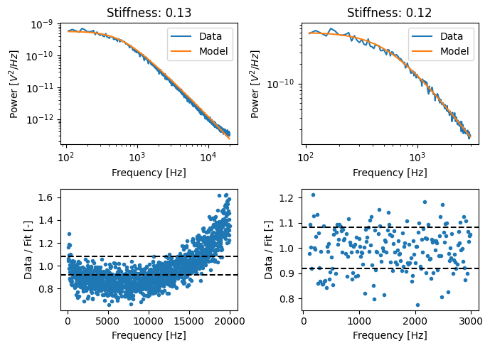
When operating at very low powers (and by extension corner frequencies), a noise floor may be visible at high frequencies. It is important to ensure that the upper limit of the fitting range does not include the noise floor as it is not taken into account in the calibration model. In the dataset below, we can see the effect of the noise floor:

lk.download_from_doi("10.5281/zenodo.7729823", "test_data")
f = lk.File("test_data/noise_floor.h5")

force_channel = f.force1x
reference_calibration = force_channel.calibration[0]
pars = {
    "force_voltage_data": force_channel.data / reference_calibration.force_sensitivity,
    "sample_rate": force_channel.sample_rate,
    "bead_diameter": 4.34,
    "temperature": 25,
    "hydrodynamically_correct": True,
    "num_points_per_block": 150,
    "fit_range": [100, 20000],
}

plt.figure(figsize=(7, 5))
plt.subplot(2, 2, 1)
calibration = lk.calibrate_force(**pars)
calibration.plot()
plt.title(f"Stiffness: {calibration.stiffness:.2f}")
plt.subplot(2, 2, 3)
calibration.plot_spectrum_residual()

plt.subplot(2, 2, 2)
calibration = lk.calibrate_force(**pars | {"fit_range": [100, 3000]})
calibration.plot()
plt.title(f"Stiffness: {calibration.stiffness:.2f}")
plt.subplot(2, 2, 4)
calibration.plot_spectrum_residual()
plt.tight_layout()

../../_images/noise_floor_free_diode.png

Note that when we have a diode calibration, excluding the noise floor becomes even more important:

diode_calibration = reference_calibration.diode_calibration
pars = pars | diode_calibration(f["Diagnostics"]["Trap power 1"])

plt.figure(figsize=(7, 5))
plt.subplot(2, 2, 1)
calibration = lk.calibrate_force(**pars)
calibration.plot()
plt.title(f"Stiffness: {calibration.stiffness:.2f}")
plt.subplot(2, 2, 3)
calibration.plot_spectrum_residual()

plt.subplot(2, 2, 2)
calibration = lk.calibrate_force(**pars | {"fit_range": [100, 3000]})
calibration.plot()
plt.title(f"Stiffness: {calibration.stiffness:.2f}")
plt.subplot(2, 2, 4)
calibration.plot_spectrum_residual()
plt.tight_layout()

../../_images/noise_floor_fixed_diode.png

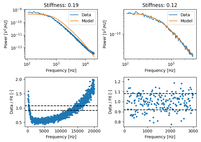
The reason the effect of the noise floor on the calibration parameters is more pronounced is because with the fixed diode model, the model is not free to adjust the diode parameters to mitigate its impact. As a result, the model uses the corner frequency in an attempt to capture the shape of the noise floor (strongly biasing the result).

Noise peaks¶

Optical tweezers are precision instruments. Despite careful determination and elimination of noise sources, it is not always possible to exclude all potential sources of noise, which can manifest in the power spectrum as spurious peaks. One downside of weighted least squares estimation, is that it is very sensitive to such outliers. It is therefore important to either exclude noise peaks from the data prior to fitting or use robust fitting. Noise peaks should always be excluded prior to blocking to minimize data loss.

Goodness of fit¶

When working with the Gaussian error model, we can calculate a goodness of fit criterion. When sufficient blocking has taken place, the sum of squared residuals that is being minimized during the fitting procedure is distributed according to a chi-squared distribution characterized by \(N_{\mathrm{dof}} = N_{\mathrm{data}} - N_{\mathrm{free}}\) degrees of freedom. Here \(N_{\mathrm{data}}\) corresponds to the number of data points we fitted (after blocking) and \(N_{\mathrm{free}}\) corresponds to the number of parameters we fitted. We can use the value we obtain to determine how unusual the fit error we obtained is.

\[\mathrm{support} = 100 P(x > \chi_{\mathrm{obtained}}^2) = 100 \int_{\chi_{\mathrm{obtained}}^2}^{\infty} \chi^2_{N_{\mathrm{dof}}}(x) dx\]

The support or backing is the probability that a repetition of the measurement that produced the data we fitted will, after fitting, produce residuals whose squared sum is greater than the one we initially obtained. More informally, it represents the probability that a fit error at least this large should occur by chance.

Support less than 1% warrants investigating the residuals for any trend in the residuals.