6. Hairpin unfolding
Download this page as a Jupyter notebook
6.1. Force-extension curve with hairpin unfolding event
In this notebook we will analyze a force-extension curve of a construct with two DNA handles with a DNA hairpin in between. The hairpin unfolds as the force on the construct is increased. A similar approach can be used to analyze force-extension curves with protein unfolding events.
First, we will compute the high frequency distance, also called piezo distance. Then, we will use the Worm-Like Chain (WLC) and Extensibly Freely Jointed Chain (EFJC) to extract the contour length of the unfolded hairpin.
6.2. Download the hairpin data
The hairpin data are stored on zenodo.org.
We can download the data directly from Zenodo using the function download_from_doi().
The data will be stored in the folder called "test_data":
filenames = lk.download_from_doi("10.5281/zenodo.12087894", "test_data")
6.3. Plot the fd curve
Before starting the analysis on the high frequency data, let’s look at fd curve based on the low frequency force, and the low frequency distance:
file = lk.File("test_data/FDCURV~3.H5")
_, fd = file.fdcurves.popitem()
plt.figure()
fd.plot_scatter()
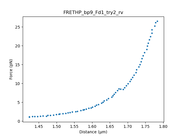
The fd curve has an unfolding event around 9 pN. We will fit the data before and after the unfolding event to determine the contour length of the hairpin.
First, we fit the video tracking to the mirror position data. The resulting fit can be used to compute the trap-to-trap distance from the (high-frequency) mirror 1 position data.
6.4. Mirror position-to-Distance Calibration
First, select the data for the mirror-to-distance calibration.:
cal_data = lk.File("test_data/FDCURV~4.H5")  # load data file with calibration"
plt.figure()
cal_data["Distance"]["Distance 1"].plot()
plt.ylabel(r"Distance ($\mu$m)")
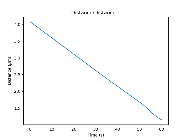
As you can see, the data becomes nonlinear for distance smaller than 1.5 micron. The ideal range for calibration is at a similar distance as used for the fd curve, but not so small that the distance becomes nonlinear. Therefore, we will choose the interval 30-40 seconds for calibration:
time_min = "30s"
time_max = "40s"
distance_calibration = lk.DistanceCalibration(
    cal_data["Trap position"]["1X"][time_min:time_max], cal_data.distance1[time_min:time_max], degree=1
)
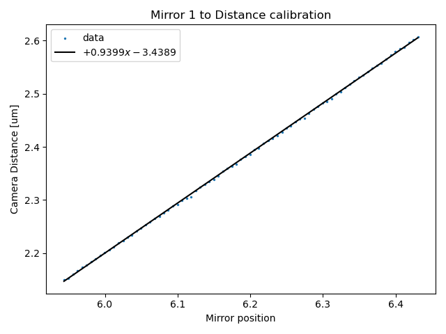
In this example, we fit a polynomial function with degree=1, which is a linear function.
Plot the result of the fit:
plt.figure()
plt.title("Mirror 1 to Distance calibration")
distance_calibration.plot()
6.5. Force Baseline Calibration
Load and plot the baseline data:
baseline_data = lk.File("test_data/FDCURV~1.H5")

baseline_1x_data = baseline_data["Force LF"]["Force 1x"]
baseline_2x_data = baseline_data["Force LF"]["Force 2x"]
distance = baseline_data["Distance"]["Distance 1"]

plt.figure()
plt.plot(distance.data, baseline_1x_data.data, label = "Baseline 1x")
plt.plot(distance.data, baseline_2x_data.data, label = "Baseline 2x")
plt.legend()
plt.ylabel("Force (pN)")
plt.xlabel(r"Distance ($\mu$m)")
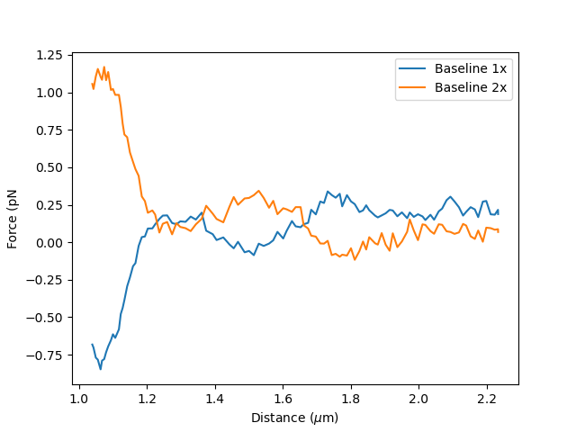
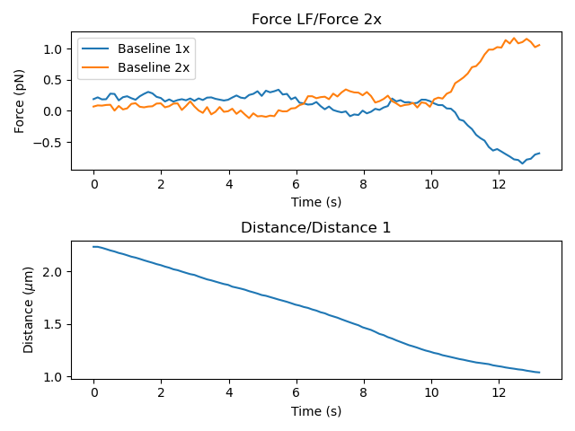
If the force was not reset before recording the baseline, it is best to subtract it before fitting. The force offset can be determined by measuring the force when the traps are far and no force is applied, which corresponds to the first seconds in the plot below:
plt.figure()
plt.subplot(2,1,1)
baseline_1x_data.plot(label = "Baseline 1x")
baseline_2x_data.plot(label = "Baseline 2x")
plt.legend()
plt.ylabel("Force (pN)")
plt.subplot(2,1,2)
distance.plot()
plt.ylabel(r"Distance ($\mu$m)")
plt.tight_layout()
Below, we average the force at large distance to estimate the distance offset:
tmin_offset = "0s"
tmax_offset = "1s"

baseline_1x_data_hf = baseline_data["Force HF"]["Force 1x"]
baseline_2x_data_hf = baseline_data["Force HF"]["Force 2x"]

f1_offset = np.mean(baseline_1x_data_hf[tmin_offset:tmax_offset].data)
f2_offset = np.mean(baseline_2x_data_hf[tmin_offset:tmax_offset].data)

baseline_1x_no_offset = baseline_1x_data_hf - f1_offset
baseline_2x_no_offset = baseline_2x_data_hf - f2_offset
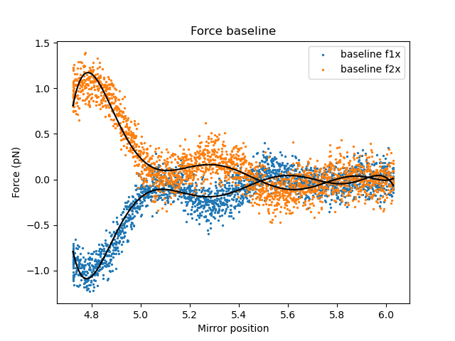
Fit the baselines using a 7th degree polynomial function:
baseline_1x = lk.ForceBaseLine.polynomial_baseline(
baseline_data["Trap position"]["1X"], baseline_1x_no_offset, degree=7, downsampling_factor=500
)
baseline_2x = lk.ForceBaseLine.polynomial_baseline(
baseline_data["Trap position"]["1X"], baseline_2x_no_offset, degree=7, downsampling_factor=500
)
Fit the result of the fit:
plt.figure()
baseline_1x.plot(label="baseline f1x")
baseline_2x.plot(label="baseline f2x")
plt.ylabel("Force (pN)")
plt.legend()
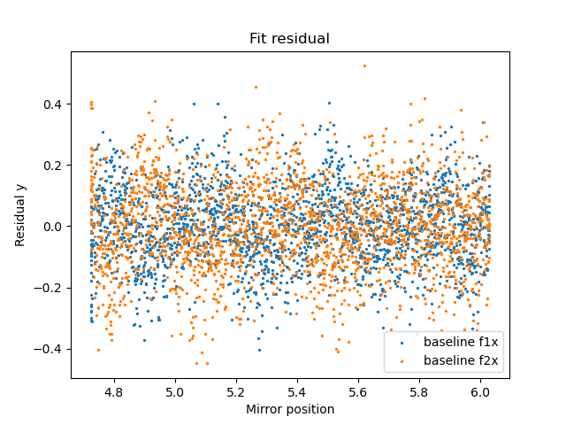
The quality of the fit can be visualized by plotting the residuals.
When the degree of the fitted polynomial is too low, the residuals will be large and not flat.:
plt.figure()
baseline_1x.plot_residual(label="baseline f1x")
baseline_2x.plot_residual(label="baseline f2x")
plt.legend(loc='lower right')
plt.show()
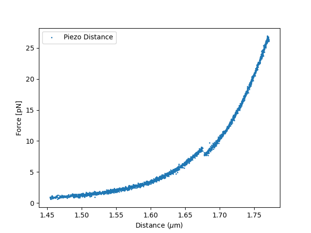
6.6. Compute the piezo distance
Now that we have determined the distance calibration and fitted the baseline, the piezo distance can be computed.
The signs parameter indicates the sign of Force 1x and Force 2x respectively. By looking at the baselines, we know that Force 1x is negative and Force 2x positive:
piezo_calibration = lk.PiezoForceDistance(distance_calibration, baseline_1x, baseline_2x, signs=(-1,1))
Choose an fd curve to compute the piezo distance for. If the force offset for the fd curve is different from the offset for the baseline, it can be included in the model. For this experiment, the offset in the baseline is also present in the fd curve. Therefore, we subtract it here:
fd_data = lk.File("test_data/FDCURV~3.H5")

tether_length, corrected_force_1x, corrected_force_2x = piezo_calibration.force_distance(
fd_data["Trap position"]["1X"], fd_data.force1x - f1_offset, fd_data.force2x - f2_offset, downsampling_factor=500
)
force_data = corrected_force_2x
Plot the result:
plt.figure()
plt.scatter(tether_length.data, force_data.data, s=1, label = "Piezo Distance")
plt.legend()
plt.xlabel(r"Distance ($\mu$m)")
plt.ylabel("Force [pN]")
6.7. Fit the data
Next, we extract the contour length of the unfolded hairpin by fitting the data before and after the unfolding event.
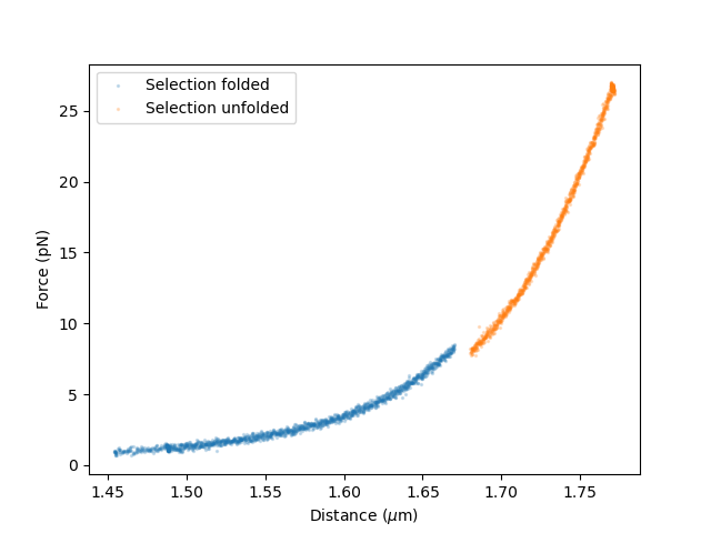
6.7.1. Data Selection
First, select data before and after the unfolding event:
def extract_fd_range(force, distance, dist_min, dist_max):
    """Extracts forces and distances for a particular distance range"""
    dist_data = distance.data
    mask = (dist_data < dist_max) & (dist_data > dist_min)
    return force.data[mask], dist_data[mask]

# Extract folded data (1.45 to 1.67 um)
force_back_folded, distance_back_folded = extract_fd_range(
    force_data, tether_length, 1.45, 1.67
)
# Extract unfolded data (1.68 to 1.8 um)
force_back_unfolded, distance_back_unfolded = extract_fd_range(
    force_data, tether_length, 1.68, 1.8
)
Plot the selected data:
plt.figure()
plt.scatter(distance_back_folded, force_back_folded,s=2,alpha=0.2,label="Selection folded")
plt.scatter(distance_back_unfolded, force_back_unfolded,s=2,alpha=0.2,label="Selection unfolded")
plt.legend()
plt.ylabel("Force (pN)")
plt.xlabel(r"Distance ($\mu$m)")
6.7.2. Define the models
For fitting the DNA handles with folded hairpin (before unfolding), the extensible Worm-Like Chain [1] is used to fit, which is valid up to 30 pN.:
dna_handles_force = lk.ewlc_odijk_force("dna_handles")
The model for DNA and the unfolded hairpin is composed by summing the model for the DNA handles and the model for the hairpin with distance as the dependent parameter. For the unfolded hairpin, we choose the Extensible Freely Jointed Chain [2], which is a variation on the Freely Jointed Chain model including the stretch modulus, to account for stretching at high forces:
dna_handles_and_hairpin_distance = lk.ewlc_odijk_distance("dna_handles") + lk.efjc_distance("dna_ss_hairpin")
Invert the model for DNA and hairpin such that force becomes the dependent parameter:
dna_handles_and_hairpin_force = dna_handles_and_hairpin_distance.invert(interpolate=True, independent_min=0, independent_max=90)
Add the models to the fit:
fit = lk.FdFit(dna_handles_force, dna_handles_and_hairpin_force)
Note that the model would look different for a protein unfolding experiment. A common model for an unfolded protein is the Worm-Like chain model, lk.wlc_marko_siggia_distance().
6.7.3. Fit the data
For fitting, we can either fit all the data at once by adding all the selected data to the fit. Another option is incremental fitting, where the DNA handles are fitted first. The fitted parameters for the DNA handles can then be used as an estimate for fitting the unfolding event. Below, we use incremental fitting.
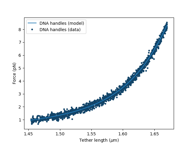
First, we add data for the DNA handles only:
fit[dna_handles_force].add_data("DNA handles",force_back_folded,distance_back_folded)
The DNA handles have a contour length of about 1.7 micron, a typical value for the persistence length of double-stranded DNA is 50 nm and a typical value for the stretch modulus is 1500 pN. Therefore, we set the initial guess of the fit as follows:
fit["dna_handles/Lp"].value = 50  # in nanometers
fit["dna_handles/Lp"].lower_bound = 30
fit["dna_handles/Lp"].upper_bound = 70
fit["dna_handles/Lc"].value = 1.7  # in microns
fit["dna_handles/St"].value = 1500  # in pN
Fit the data before unfolding:
fit.fit()
Plot the result of the fit:
plt.figure()
fit[dna_handles_force].plot()
plt.xlabel(r"Distance ($\mu$m)")
plt.ylabel("Force (pN)")
Now, add the data after the unfolding event:
fit[dna_handles_and_hairpin_force].add_data("DNA handles + unfolded hairpin",force_back_unfolded,distance_back_unfolded)
This time all the selected data are fitted and the values for the DNA handles from the first part of the fit are used as initial guess.
Sometimes, when fitting many unfolding events, the fit does not converge well when all data are fitted at once. If that happens, you can fix parameters from the first fit at this stage, for example by setting
fit["dna_handles/Lc"].fixed = True. For this particular data set, the fit converges without fixing parameters.
We next set the initial guesses for the unfolded hairpin:
fit["dna_ss_hairpin/Lp"].lower_bound = 0.5  # in nanometers
fit["dna_ss_hairpin/Lp"].value = 1.5
fit["dna_ss_hairpin/Lp"].upper_bound = 2.0

fit["dna_ss_hairpin/Lc"].value = 0.02  # in microns
fit["dna_ss_hairpin/Lc"].lower_bound = 0.001

fit["dna_ss_hairpin/St"].value = 500  # in pN
fit["dna_ss_hairpin/St"].upper_bound = 2000
Fit all the data and plot the result:
>>> fit.fit()
>>> print(fit.params)
Name                  Value       Unit      Fitted   Lower bound    Upper bound
--------------      ------------ --------  -------  -------------  -------------
dna_handles/Lp        34.7309    [nm]        True    30              100
dna_handles/Lc         1.75753   [micron]    True     0.00034        inf
dna_handles/St       904.301     [pN]        True     1              inf
kT                     4.11      [pN*nm]     False    3.77           8
dna_ss_hairpin/Lp      0.785985  [nm]        True     0.5            2
dna_ss_hairpin/Lc      0.0215748 [micron]    True     0.001          inf
dna_ss_hairpin/St   2000         [pN]        True     1              2000
As can be seen from the table, most fitted parameters converge and have values in the expected range. However, the stretch modulus of the hairpin hits the upper bound of 2000 pN, indicating that this parameter did not converge.
When observing that a parameter does not converge, it is important to go back to the fit and see how it can be improved. In this case, increasing the upper bound for dna_ss_hairpin/St does not visually change the fit and does not result in convergence;
the stretch modulus of the DNA handles and the hairpin cannot be optimized at the same time. A solution would be to use the freely jointed chain, instead of the extensible freely jointed chain to fit the unfolded hairpin, which is equivalent to setting
a very large value for dna_ss_hairpin/St:
fit["dna_ss_hairpin/St"].upper_bound = 100000  # in pN
fit["dna_ss_hairpin/St"].value = 100000
fit["dna_ss_hairpin/St"].fixed = True
fit.fit()
Plot the result:
plt.figure()
fit[dna_handles_force].plot()
fit[dna_handles_and_hairpin_force].plot()
plt.xlabel(r"Distance ($\mu$m)")
plt.ylabel("Force (pN)")
Lc_hairpin = fit["dna_ss_hairpin/Lc"].value*1000
plt.title(f"Fitted hairpin length is {Lc_hairpin:0.1f} nm")
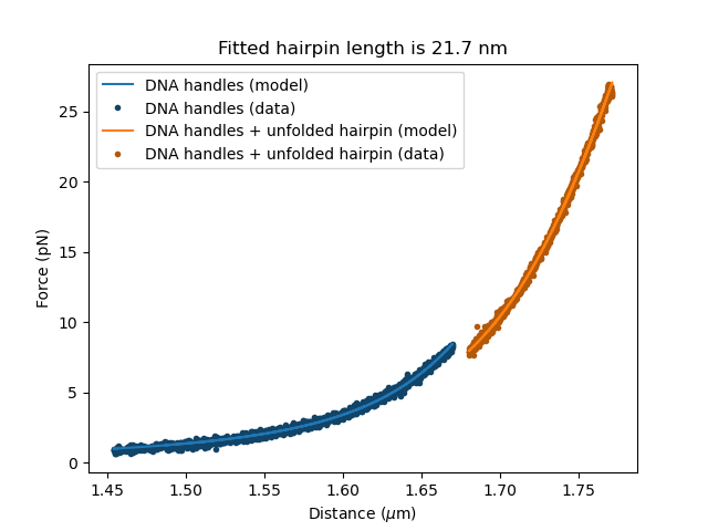
The expected contour length for the hairpin was ~17 nm and the fitted length is 21.7 nm.
6.7.4. Check and improve fit quality
The next step is to study the confidence intervals and quality of the fit, for example using the likelihood profile. The fit can be improved further by fitting multiple data sets at once. For more information on this procedure, see the section on global fitting.
6.7.5. Unequal bead sizes
In this example, the two bead sizes are equal. Since this is the case, we used a single template to track the bead positions. This means that even if a template is not centered perfectly, any offset negates, because both templates are offset in an identical manner. When using different beads however, one uses two different templates, which means that an offset from one template is not automatically cancelled by the other template. As a result, we can end up with an offset in the bead-to-bead distance due to a slight off-centering of one or both of the templates. When working with unequal bead sizes, an extra distance offset can be included in the model to account for not perfectly centered templates.
When fitting, the contour length and distance offset are strongly correlated and can often not be optimized at the same time, as explained here. A common solution is to fix the known contour length of the DNA handles during fitting.