Surface proximity

Download this page as a Jupyter notebook

The theory in the previous section holds for beads far away from any surface (in bulk). When doing experiments near the surface, the surface starts to have an effect on the friction felt by the bead. When the height and bead radius are known, the hydrodynamically correct model can take this into account.

The hydrodynamically correct model works well when the bead center is at least 1.5 times the radius above the surface. When moving closer than this limit, it is better to use a model that more accurately describes the change in drag at low frequencies, but neglects the frequency dependent effects.

To see why this is, consider model predictions for the drag coefficient at frequency zero (constant flow). At frequency zero, the Lorentzian and hydrodynamically correct model should predict similar behavior (as the hydrodynamic effects should only be present at higher frequencies). Let’s compare the difference between the simple Lorentzian model and the hydrodynamically correct model near the surface:

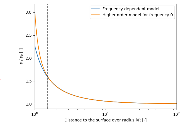
where \(l\) is the distance between the bead center and the surface and \(R\) is the bead radius.

In addition, the frequency dependent effects reduce as we approach the surface [SchafferNorrelykkeH07]. We can see this when we plot the spectrum for two different ratios of l/R.

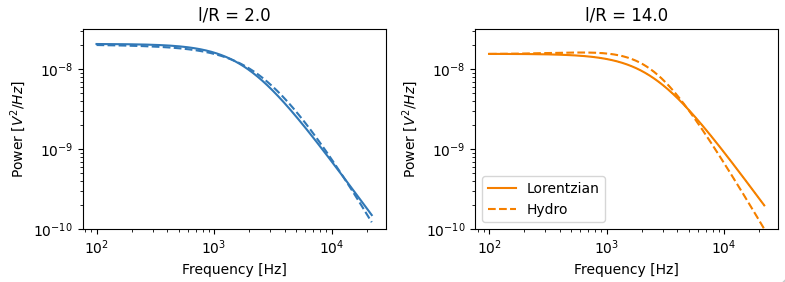
These two aspects make using the simpler model in combination with a Lorentzian a more suitable model for situations where we have to calibrate extremely close to the surface.

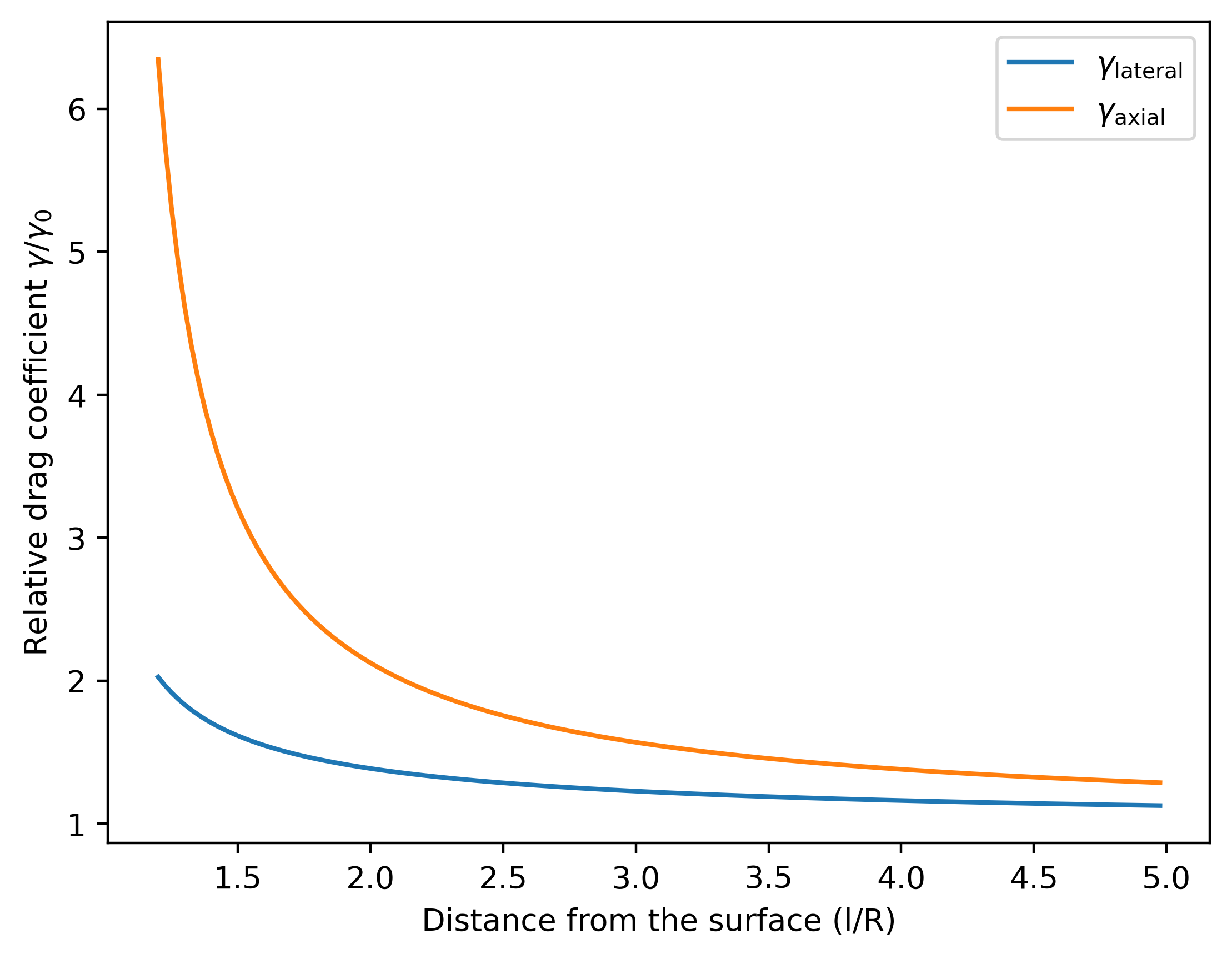
Lastly, note that the height-dependence of _axial_ force is different than the height-dependence of lateral force. For axial force, no hydrodynamically correct theory for the power spectrum near the surface exists.

Mathematical background

Hydrodynamically correct theory

When approaching the surface, the drag experienced by the bead depends on the distance between the bead and the surface of the flow cell. An approximate expression for the frequency dependent drag is then given by [TolicNorrelykkeSchafferH+06]:

\[\gamma(f, R/l) = \frac{\gamma_\mathrm{stokes}(f)}{1 - \frac{9}{16}\frac{R}{l} \left(1 - \left((1 - i)/3\right)\sqrt{\frac{f}{f_{\nu}}} + \frac{2}{9}\frac{f}{f_{\nu}}i - \frac{4}{3}(1 - e^{-(1-i)(2l-R)/\delta})\right)} \tag{$\mathrm{kg/s}$}\]

Where \(\delta = R \sqrt{\frac{f_{\nu}}{f}}\) represents the penetration depth, \(R\) corresponds to the bead radius and \(l\) to the distance from the bead center to the nearest surface.

While these models may look daunting, they are all available in Pylake and can be used by simply providing a few additional arguments to the PassiveCalibrationModel. It is recommended to use these equations when less than 10% systematic error is desired [TolicNorrelykkeSchafferH+06]. No general statement can be made regarding the accuracy that can be achieved with the simple Lorentzian model, nor the direction of the systematic error, as it depends on several physical parameters involved in calibration [BSPW+06, TolicNorrelykkeSchafferH+06].

Note

One thing to note is that when considering the surface in the calibration procedure, the drag coefficient returned from the model corresponds to the drag coefficient extrapolated back to its bulk value.

Lorentzian model (lateral)

The hydrodynamically correct model presented in the previous section works well when the bead center is at least 1.5 times the radius above the surface. When moving closer than this limit, we fall back to a model that more accurately describes the change in drag at low frequencies, but neglects the frequency dependent effects.

To understand why, let’s introduce Faxen’s approximation for drag on a sphere near a surface under creeping flow conditions. This model is used for lateral calibration very close to a surface [SchafferNorrelykkeH07] and is given by the following equation:

\[\gamma_\mathrm{faxen}(R/l) = \frac{\gamma_0}{ 1 - \frac{9R}{16l} + \frac{1R^3}{8l^3} - \frac{45R^4}{256l^4} - \frac{1R^5}{16l^5} } \tag{$\mathrm{kg/s}$}\]

What we see is that the frequency dependent model used in the previous section reproduces this model up to and including its second order term in \(R/l\). It is, however, a lower order model and the accuracy decreases rapidly as the distance between the bead and surface become very small.

Lorentzian model (axial)

For calibration in the axial direction, no hydrodynamically correct theory exists.

Similarly as for the lateral component, we will fall back to a model that describes the change in drag at low frequencies. However, while we had a simple expression for the lateral drag as a function of distance, no simple closed-form equation exists for the axial dimension. Brenner et al provide an exact infinite series solution [Bre61]. Based on this solution [SchafferNorrelykkeH07] derived a simple equation which approximates the distance dependence of the axial drag coefficient.

\[\gamma_\mathrm{axial}(R/l) = \frac{\gamma_0}{ 1.0 - \frac{9R}{8l} + \frac{1R^3}{2l^3} - \frac{57R^4}{100l^4} + \frac{1R^5}{5l^5} + \frac{7R^{11}}{200l^{11}} - \frac{1R^{12}}{25l^{12}} } \tag{$\mathrm{kg/s}$}\]

This model deviates less than 0.1% from Brenner’s exact formula for \(l/R >= 1.1\) and less than 0.3% over the entire range of \(l\) [SchafferNorrelykkeH07].