Active Calibration

For certain applications, passive force calibration, as described above, is not sufficiently accurate. Using active calibration, the accuracy of the calibration can be improved. The reason for this is that active calibration uses fewer assumptions than passive calibration.

When performing passive calibration, we base our calculations on a theoretical drag coefficient. This theoretical drag coefficient depends on parameters that are only known with limited precision:

• The diameter of the bead \(d\) in microns.

• The dynamic viscosity \(\eta\) in Pascal seconds.

• The distance to the surface \(h\) in microns.

This viscosity in turn depends strongly on the local temperature around the bead, which depends on several physical parameters (e.g. the power of the trapping laser, the buffer medium, the bead size and material) and is typically poorly known.

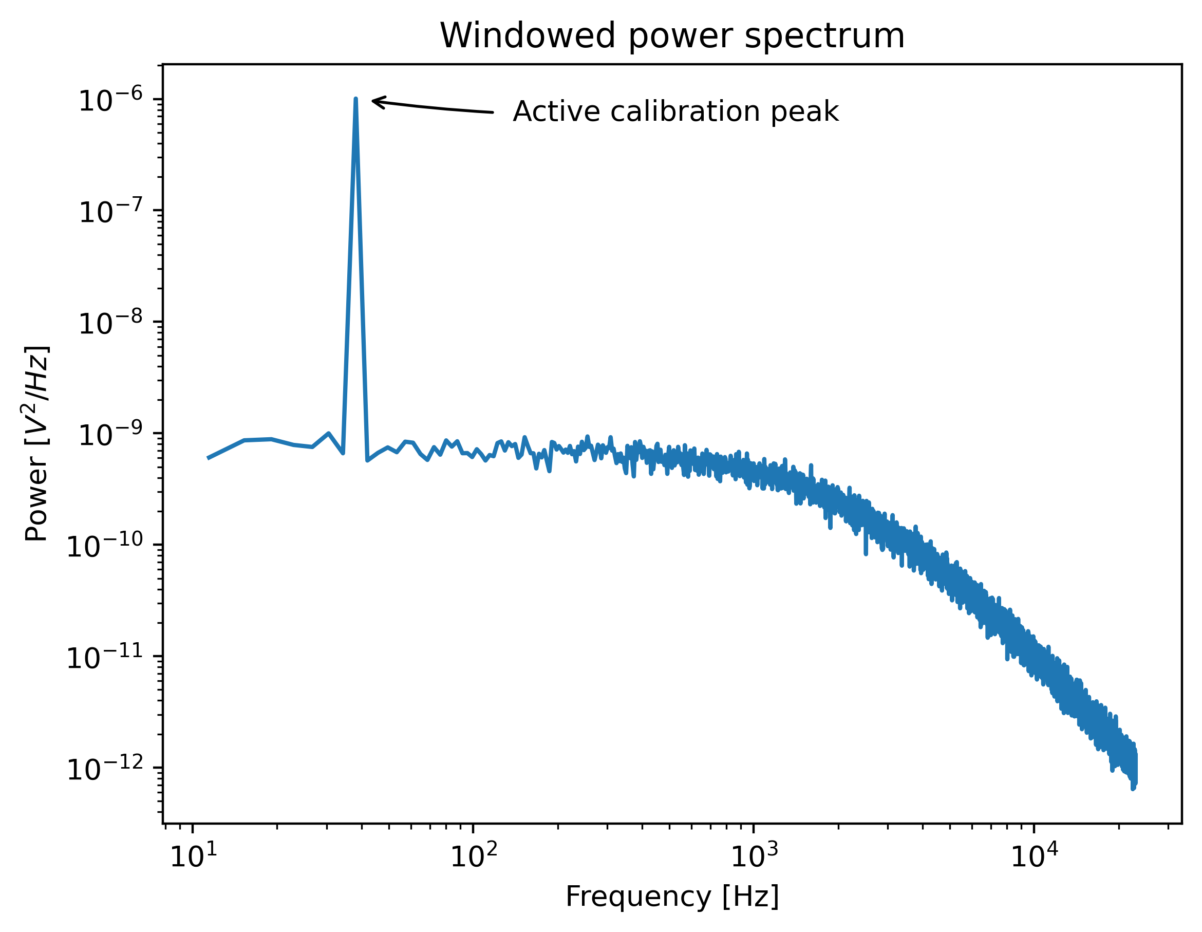
During active calibration, the trap or nanostage is oscillated sinusoidally. These oscillations result in a driving peak in the force spectrum. Using power spectral analysis, the force can then be calibrated without prior knowledge of the drag coefficient.

When the power spectrum is computed from an integer number of oscillations, the driving peak is visible at a single data point at \(f_\mathrm{drive}\).

The physical spectrum is then given by a thermal part (like before):

\[P^\mathrm{thermal}(f) = \frac{D}{\pi ^ 2 \left(f^2 + f_c^2\right)} \tag{$\mathrm{m^2/Hz}$}\]

And an active part:

\[P^\mathrm{active}(f) = \frac{A^2}{2\left(1 + \frac{f_c^2}{f_\mathrm{drive}^2}\right)} \delta(f - f_\mathrm{drive}) \tag{$\mathrm{m^2/Hz}$}\]

Here \(A\) refers to the driving amplitude. Added together, these give rise to the full power spectrum:

\[P^\mathrm{total}(f) = P^\mathrm{thermal}(f) + P^\mathrm{active}(f) \tag{$\mathrm{m^2/Hz}$}\]

Since we know the driving amplitude, we know how the bead reacts to the driving motion and we can observe this response in the power spectrum, we can use this relation to determine the positional calibration.

If we use the basic Lorentzian model, then the theoretical power (integral over the delta spike) corresponding to the driving input is given by [TolicNorrelykkeSchafferH+06]:

\[W_\mathrm{physical} = \frac{A^2}{2\left(1 + \frac{f_c^2}{f_\mathrm{drive}^2}\right)} \tag{$\mathrm{m^2}$}\]

Subtracting the thermal part of the spectrum, we can determine the same quantity experimentally.

\[W_\mathrm{measured} = \left(P_\mathrm{measured}^\mathrm{total}(f_\mathrm{drive}) - P_\mathrm{measured}^\mathrm{thermal}(f_\mathrm{drive})\right) \Delta f \tag{$\mathrm{V^2}$}\]

where \(\Delta f\) refers to the width of one spectral bin. Here the thermal contribution that needs to be subtracted is obtained from fitting the thermal part of the spectrum using the passive calibration procedure from before. The desired positional calibration is then:

\[R_d = \sqrt{\frac{W_\mathrm{physical}}{W_\mathrm{measured}}} \tag{$\mathrm{m/V}$}\]

Note how this time around, we did not rely on assumptions on the viscosity of the medium or the bead size.

As a side effect of this calibration, we actually obtain an experimental estimate of the drag coefficient:

\[\gamma_\mathrm{measured} = \frac{k_B T}{R_d^2 D_\mathrm{measured}} \tag{$\mathrm{kg/s}$}\]

Analogously to passive calibration, there is also a hydrodynamically correct theory for active calibration which should be used when inertial forces cannot be neglected. This involves fitting the thermal spectrum with the hydrodynamically correct power spectrum discussed earlier, but also requires using a hydrodynamically correct model for the peak:

\[P_\mathrm{hydro}^\mathrm{active}(f) = \frac{\left(A f_\mathrm{drive} \left|\gamma / \gamma_0\right|\right)^2 \delta \left(f - f_\mathrm{drive}\right)}{2 \left(\left(f_{c,0} + f \mathrm{Im}(\gamma/\gamma_0) - f^2/f_{m, 0}\right)^2 + \left(f \mathrm{Re}(\gamma / \gamma_0)\right)^2\right)} \tag{$\mathrm{m^2/Hz}$}\]

We can also include a distance to the surface like before. This results in an expression for the drag coefficient \(\gamma\) that depends on the distance to the surface which is given by the same equations as listed in the section on the hydrodynamically correct model.