Pylake 1.2.0

Pylake v1.2.0 has been released with new features and improvements to existing analyses. Here’s some of the highlights:

Improved binding time analysis

Correctly use the minimum observable time in dwell time analysis

In earlier versions of Pylake, binding time analysis would return biased estimates when analyzing kymographs with very few events. This was because fit_binding_times() relied on the assumption that the shortest track in the KymoTrackGroup represented the minimum observable dwell time. This assumption is likely valid for kymographs with many tracks but problematic when few events occur per kymograph. In this case, binding times will be underestimated. For more information see the changelog.

Important

The old (incorrect) behavior is maintained as default until the next major release (v2.0.0) to ensure backward compatibility. To enable the fixed behavior, specify observed_minimum=False when calling fit_binding_times().

Note that CSVs exported from the kymotracker widget before v1.2.0 will contain insufficient metadata to make use of the improved analysis. To create this metadata, use filter_tracks() on the group with a specified min_length before further analysis. CSVs exported starting from v1.2.0 contain an additional data column with this data under the header "minimum_length (-)".

Correct for discretization in binding lifetime analysis

You can now take into account the discretized nature of observed binding times of tracked particles. When lifetimes are short (compared to the scan line time) this can significantly improve results by removing bias from the fitted lifetimes. Simply use discrete_model=True with fit_binding_times().

Plot KymoTrack Gaussian fit

You can now easily plot the fitting results from refine_tracks_gaussian() for a particular scan line using KymoTrack.plot_fit() or KymoTrackGroup.plot_fit().

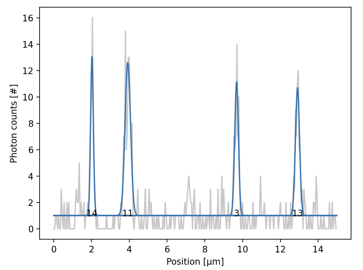
Gaussian fits to signal peaks along a scan line of a tracked kymograph.

Refine gaussian simultaneous

The new fitting mode "simultaneous" was introduced to refine_tracks_gaussian() which enforces optimization bounds between peak positions when two tracks are close together. This ensures that individual gaussians cannot switch positions between two tracks (which was a faulty behavior that could occur using the previous “multiple” method). For more information see the changelog.

Important

The fitting mode "simultaneous" is the recommended flag for refining tracks that may be close together. The previous "multiple" option is deprecated and will be removed in a future release.

Generate colormaps according to emission wavelength

By default, single-channel images arising from fluorophores excited with the red, green, and blue lasers are plotted with the corresponding ~lumicks.pylake.colormaps.red lk.colormaps.red, lk.colormaps.green, and lk.colormaps.blue colormaps, respectively. However, the actual light emitted is always red-shifted from the excitation color. Now you can plot single-channel images with the approximate color of the signal emitted based on the emission wavelength using the from_wavelength() method of colormaps.

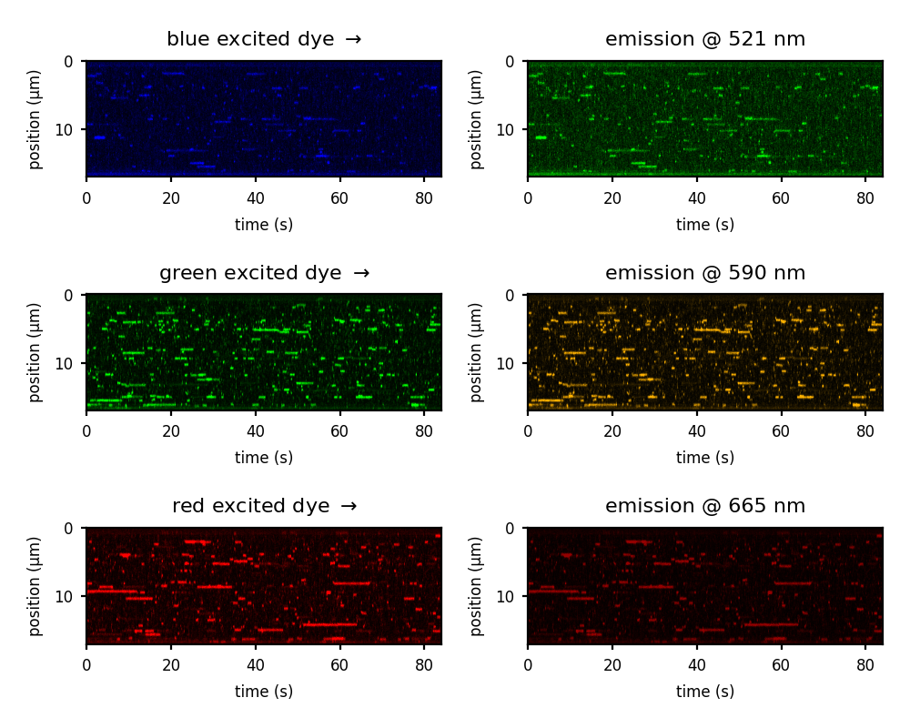
Kymographs showing tracks in three color channels using the default colormaps (left) and colormaps corresponding to the actual emission colors (right).

Robust force calibration

Added a new fitting method to deal with spurious noise peaks in power spectra during force calibration. See the Force Calibration tutorial for more details!

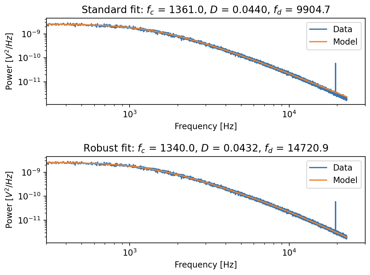
Fitting a power spectrum with a noise peak at ~20,000 Hz. Top panel: using the standard passive calibration, we can see that the fit is skewed at high frequency end. Bottom panel: using the robust fitting method, the skewness is removed.

Cropping h5 files

You can now use lk.File.save_as(crop_time_range=(start_timestamp, stop_timestamp)) to export a specific time range to a new h5 file. This can be useful for when you want to export a specific part of the timeline or a partial kymograph for instance. Exporting a partial file helps keep file size down and makes it easier to share only the relevant parts of your data with others.