10. Population Dynamics
Download this page as a Jupyter notebook
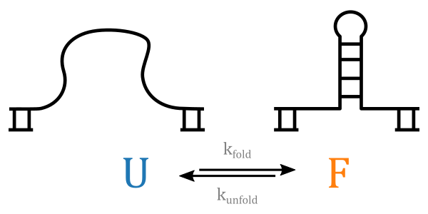
The following tools enable analysis of experiments which can be described as a system of discrete states. Consider as an example a DNA hairpin which can exist in a folded and unfolded state. At equilibrium, the relative populations of the two states are governed by the interconversion kinetics described by the rate constants \(k_{fold}\) and \(k_{unfold}\)
First let’s take a look at some example force channel data. We’ll downsample the data in order to speed up the calculations and smooth some of the noise:
raw_force = file.force1x
force = raw_force.downsampled_by(78)

raw_force.plot()
force.plot(start=raw_force.start)
plt.xlim(0, 3)
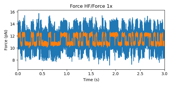
Care must be taken in downsampling the data so as not to introduce signal artifacts in the data (see below for a more detailed discussion).
The goal of the analyses described below is to label each data point in a state in order to extract kinetic and thermodynamic information about the underlying system.
10.1. Gaussian Mixture Models
The Gaussian Mixture Model (GMM) is a simple probabilistic model that assumes all data points belong to one of a fixed number of states, each of which is described by a (weighted) normal distribution.
We can initialize a model from a force channel as follows:
gmm = lk.GaussianMixtureModel.from_channel(force, n_states=2)
print(gmm.weights) # [0.53070846 0.46929154]
print(gmm.means)   # [10.72850757 12.22295543]
print(gmm.std)     # [0.21461742 0.21564235]
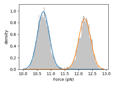
Here the force data is used to train a 2 state GMM. The weights give the fraction of time spent each state while the means and standard deviations indicate the average signal and noise for each state, respectively.
We can visually inspect the quality of the fitted model by plotting a histogram of the data overlaid with the weighted normal distribution probability density functions:
gmm.hist(force)
We can also plot the time trace with each data point labeled with the most likely state:
gmm.plot(force['0s':'2s'])

Note that the data does not have to be the same data used to train the model.
10.1.1. Data Pre-processing
It can be desirable to downsample the raw channel data in order to decrease the number of data points used by the model training algorithm (in order to speed up the calculation) and to smooth experimental noise. However, great care must be taken in doing so in order to avoid introducing artifacts into the signal.
As shown in the histograms below, as the data is downsampled the state peaks narrow considerably, but density between the peaks remains (indicated by the arrow). These intermediate data points are the result of averaging over a span of data from two different states. The result is the creation of a new state that does not arise from any physically relevant mechanism.
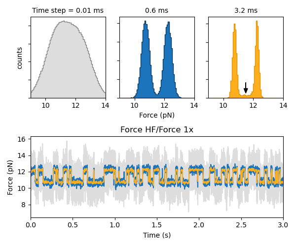
Furthermore, states with very short lifetimes can be averaged out of the data if the downsampling factor is too high. Therefore, in order to ensure robust results, it may be advisable to carry out the analysis at a few different downsampled rates.
10.2. Dwell time analysis
The lifetimes of bound states can be estimated by fitting observed dwell times \(t\) to a mixture of Exponential distributions.
where each of the \(M\) exponential components is characterized by a lifetime \(\tau_i\) and an amplitude (or fractional contribution) \(a_i\) under the constraint \(\sum_i a_i = 1\). The lifetime describes the mean time a state is expected to persist before transitioning to another state. The distribution can alternatively be parameterized by a rate constant \(k_i = 1 / \tau_i\).
The DwelltimeModel class can be used to optimize the model parameters for an array of determined dwell times:
dwell_1 = lk.DwelltimeModel(dwelltimes_seconds, n_components=1)
The model is optimized using Maximum Likelihood Estimation (MLE) [KJC+19, WLG+16]. The advantage of this method
is that it does not require binning the data. The number of exponential components to be used for the fit is chosen with the n_components argument.
The optimized model parameters can be accessed with the lifetimes and amplitudes
properties. In the case of first order kinetics, the rate constants can be accessed with the rate_constants property.
This value is simply the inverse of the optimized lifetime(s). See Assumptions and limitations on determining rate constants for more information.
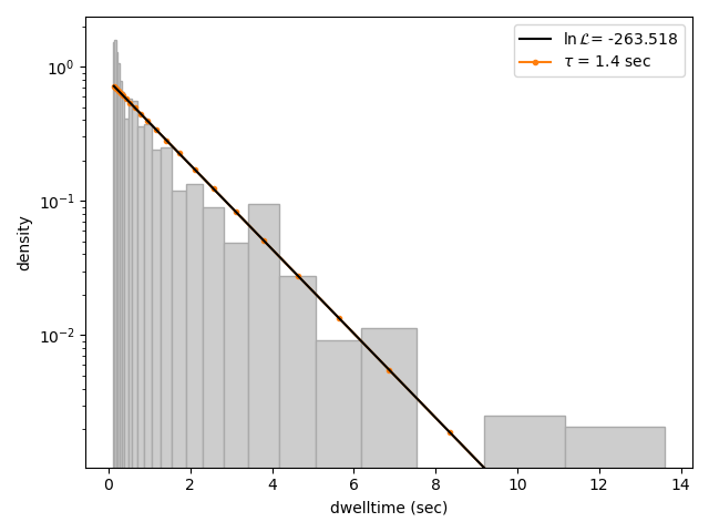
We can visually inspect the result with:
dwell_1.plot(bin_spacing="log")
The bin_spacing argument can be either "log" or "linear" and controls the spacing of the bin edges.
The scale of the x- and y-axes can be controlled with the optional xscale and yscale arguments; if they are not specified
the default visualization is lin-lin for bin_spacing="linear" and lin-log for bin_spacing="log". You can also optionally pass the number of
bins to be plotted as n_bins.
Note
The number of bins is purely for visualization purposes; the model is optimized directly on the unbinned dwell times. This is the main advantage of the MLE method over analyses that use a least squares fitting to binned data, where the bin widths and number of bins can drastically affect the optimized parameters.
We can clearly see that this distribution is not fit well by a single exponential decay. Let’s now see what a double exponential distribution looks like:
dwell_2 = traces.fit_binding_times(n_components=2)
dwell_2.plot(bin_spacing="log")
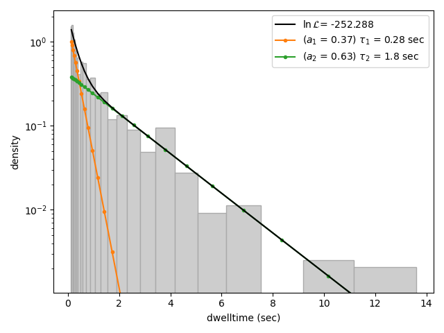
Here we see that the double exponential fit visually looks better and the log likelihood is also higher than that for the single exponential fit. However, the log likelihood does not take into account model complexity, and will always increase for a model with more degrees of freedom. Instead, we can look at the Bayesian Information Criterion (BIC) or Akaike Information Criterion (AIC) to determine which model is better:
>>> print(dwell_1.bic, dwell_1.aic)
532.3299315589168  529.0366267341923

>>> print(dwell_2.bic, dwell_2.aic)
520.4562630650156  510.5763485908421
These information criterion values weigh the log likelihood against the model complexity, and as such are more useful for model selection. In general, the model with the lowest value is optimal. We can see that both values are lower for the double exponential model, indicating that it is a better fit to the data.
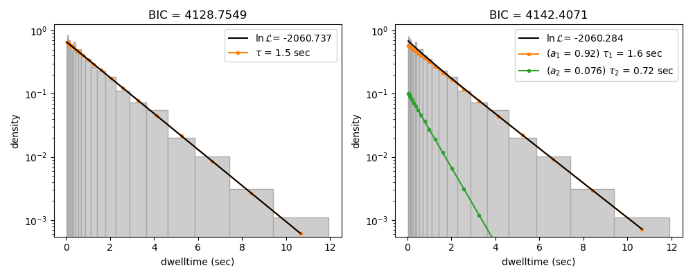
We can see this effect if we purposely overfit the data. The following plot shows the result of fitting simulated data (randomly sampled from a single exponential distribution) with either a one- or two-component model. In the figure legends we see that the log likelihood increases slightly for the two-component model because of the larger degrees of freedom. However, the BIC for the one-component model is indeed lower, as expected:
Going back to our experimental data, we can next attempt to estimate confidence intervals (CI) for the parameters using bootstrapping. Here, a random dataset with the same size as the original is sampled (with replacement) from the original dataset. This sampled dataset is then fit using the MLE method, just as for the original dataset. The fit results in a new estimate for the model parameters. This process is repeated many times, and the distribution of the resulting parameters can be analyzed to estimate certain statistics about the them:
dwell_2.calculate_bootstrap(iterations=1000)
dwell_2.bootstrap.plot(alpha=0.05)
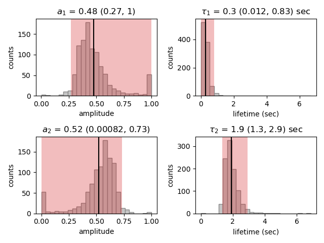
Here we see the distributions of the bootstrapped parameters. The vertical lines indicate the
means of the distributions, while the red area indicates the estimated confidence intervals. The alpha argument determines
the CI that is estimated as 100*(1-alpha) % CI; in this case we’re showing the estimate for the 95% CI. The values for the
lower and upper bounds are the 100*(alpha/2) and 100*(1-alpha/2) percentiles of the distributions.
Note, however, that while the means correspond well with the optimized model parameters, the distributions are not symmetric.
In such a case, the simple method of using percentiles as CI values may not be appropriate. For more advanced analysis,
the distribution values are directly available through the properties DwelltimeModel.bootstrap.amplitude_distributions and
DwelltimeModel.bootstrap.lifetime_distributions which return the data as a numpy array with
shape [# components, # bootstrap samples].
10.2.1. Assumptions and limitations on determining rate constants
When using an exponential distribution to model biochemical kinetics, care must be taken to ensure that the model appropriately describes the observed system. Here we briefly describe the underlying assumptions and limitations for using this method.
The exponential distribution describes the expected dwell times for states in a first order reaction where the rate of transitioning from the state is dependent on the concentration of a single component. A common example of this is the dissociation of a bound protein from a DNA strand:
This reaction is characterized by a rate constant \(k_\mathrm{off}\) known as the dissociation rate constant with units of \(\mathrm{sec}^{-1}\).
Second order reactions which are dependent on two reactants can also be determined in this way if certain conditions are met. Specifically, if the concentration of one reactant is much greater than that of the other, we can apply the first order approximation. This approximation assumes the concentration of the more abundant reactant remains approximately constant throughout the experiment and therefore does not contribute to the reaction rate. This condition is often met in single-molecule experiments; for example in a typical C-Trap experiment, the concentration of a protein in solution on the order of nM is significantly higher than the concentration of the single trapped tether.
A common example of this is the binding of a protein to a DNA strand:
This reaction is described by the second order association rate constant \(k_\mathrm{on}\) with units of \(\mathrm{M}^{-1}\mathrm{sec}^{-1}\). Under the first order approximation, this can be determined by fitting the appropriate dwell times to the exponential model and dividing the resulting rate constant by the concentration of the protein in solution.
Note
The calculation of \(k_\mathrm{on}\) relies on having an accurate measurement of the bulk concentration. Care should be taken as this can be difficult to determine when working in the nanomolar regime, as nonspecific adsorption can lower the effective concentration at the experiment.
10.2.2. A warning on reliability and interpretation of multi-exponential kinetics
Sometimes a process can best be described by two or more exponential distributions. This occurs when a system consists of multiple states with different kinetics that emit the same observable signal. For instance, the dissociation rate of a bound protein might depend on the microscopic conformation of the molecule that does not affect the emission intensity of an attached fluorophore used for tracking. Care must be taken when interpreting results from a mixture of exponential distributions.
However, in the setting of a limited number of observations, the optimization of the exponential mixture can become non-identifiable, meaning that there are multiple sets of parameters that result in near equal likelihoods. A good first check on the quality of the optimization is to run a bootstrap simulation (as described above) and check the shape of the resulting distributions. Very wide, flat, or skewed distributions can indicate that the model was not fitted to a sufficient amount of data. For processes that are best described by two exponentials, it may be necessary to acquire more data to obtain a reliable fit.
10.2.3. The Exponential (Mixture) Model
The model likelihood \(\mathcal{L}\) to be maximized is defined for a mixture of exponential distributions as:
where \(T\) is the number of observed dwell times, \(M\) is the number of exponential components, \(t\) is time, \(\tau_i\) is the lifetime of component \(i\), and \(a_i\) is the fractional contribution of component \(i\) under the constraint of \(\sum_i^M a_i = 1\). The normalization constant \(N\) is defined as:
where \(t_{min}\) and \(t_{max}\) are the minimum and maximum possible observation times.
The normalization constant takes into account the minimum and maximum possible observation times of the experiment. These
can be set manually with the min_observation_time and max_observation_time keyword arguments, respectively. The default
values are \(t_{min}=0\) and \(t_{max}=\infty\), such that \(N=1\). However, for real experimental data,
there are physical limitations on the measurement times (such as pixel integration time for kymographs or sampling frequency for
force channels) that should be taken into account.